Final Report
Contents |
1 Introduction
1.1 List of contributors
Editors: A.J. Illingworth, D. Ruffieux, D. Cimini, U. Löhnert, M. Haffelin, V. Lehmann.
Contributors (in alphabetical order): F. Angelini, E. Batchvarova, C. Brandau, D. Cimini, O. Cox, H. Czekala, A. Dabas, D. Donovan, J.C. Dupont, K. Ebell, J. Fernández-Gálvez, M. E. Ferrario, C. Gaffard, G.P. Gobbi, U. Görsdorf, J. Güldner, A. Haefele, M. Haffelin, F. Hurter, A.J. Illingworth, S. Kauczok, H. Klein Baltink, V. Lehmann, R. Lehtinen, D. Leuenberger, U. Löhnert, S. Lolli, F. Madonna, O. Maier, G. Martucci, G. Maschwitz, I. Mattis, D. Nicolae, E. O’Connor, G. Pace, S. Pal, M. Piringer, B. Pospichal, D. Ruffieux, L. Sauvage, B. Thies, L. Thobois, W. Thomas, M. Wiegner.
1.2 General Remarks
The advent of high resolution climate models together with high resolution weather forecast models running at global, regional and 1km convection resolving scales requires an integrated composite observing sytem which builds on existing infrastructure.Such a system must be of appropriate quality to meet the requirements of the numerical weather prediction (NWP) and climate coummunity. The goal of the COST action ES0702 is to specify an optimum European network of inexpensive, unmanned ground based profiling stations, which can provide continuous profiles of winds, humidity, temperature, clouds and aerosol properties.
If the data from these networks are to be used, then several conditions must be fulfilled. Firstly a standard calibration, maintenance, and automatic data quality checking system must be developed. Secondly, the format of the data must be the same, so that it can be exchanged efficiently and rapidly in near real time. The model can then be evaluated by comparison with the observations over over a suitably long period. Ideally difficulties with the model can be identified and rectified so we can move to the third stage, and the 'O-B' statistics can be derived. That is to say the statistics of the difference between the observation and the background state. If the absence of bias can be confirmed, the standard deviations of the differences characterised and the spatial representativity of the observations established, then the observations can be considered as candidates for data assimilation and they can be used to improve the initial state of the model so that it better represents the true state of the atmosphere. The density of the network is a balance between the spatial representativity of the observations and the economic costs of deploying the instruments.
This document provides a summary of the major findings and conclusions of the EG-CLIMET action. It highlights four profiling instruments, their synergy, and NWP applications. The instruments provide profiles of aerosol and cloud backscatter, winds, temperature and humidity:
- Ceilometers
- Doppler lidars,
- Wind profilers
- Microwave Radiometers
- Synergy and NWP applications
1.3 Summary of Findings and Recommendations
Ceilometers: EG-CLIMET has
- Compiled a list of hundreds of ceilometers deployed in Europe.
- Demonstrated they could supply real time backscatter profiles from clouds and aerosols.
- Demonstrated simple accurate calibration techniques using atmospheric targets
- Demonstrated they can measure the boundary layer height in unstable boundary layers.
- Compared the backscatter profiles of clouds and aerosols with NWP models predictions.
- Recommended to EUCOS that these instruments be networked to provide real time data.
Doppler Lidars: EG-CLIMET has
- Examined the performance of new Doppler lidars; 25 are now deployed in Europe.
- Demonstrated that they can provide accurate winds in the boundary layer.
- Demonstrated they can measure turbulence and vertical exchange in the boundary layer.
- Recommended to EUCOS that these instruments be networked to provide real time data.
Wind Profilers: EG-CLIMET has
- Developed algorithms, now implemented operationally, to reject spurious bird echoes.
- Improved algorithms, now implemented operationally, for rejecting spurious ground clutter.
- Demonstrated the positive impact of well-maintained wind profilers on NWP forecasts.
Microwave Radiometers: EG-CLIMET has
- Compiled a list of MWRs in Europe and developed an international network: MWRnet.
- Demonstrated the accuracy of temperature and water vapour in retrieved profiles.
- Demonstrated the value of MWR in estimating boundary layer depth.
- Provided the first comparison of MWR retrievals with NWP model predictions.
Synergy and NWP: EG-CLIMET has shown that
- Ceilometer data may be used for evaluation of NWP models and subsequent assimilation.
- Doppler Lidars, together with Wind Profilers, can provide winds throughout the troposphere.
- Strategically placed wind profilers have a positive impact on NWP forecasts.
- Wind profilers are operationally assimilated in several NWP models. Moreover, they can be combined with NWP to provide warnings in case of a nuclear hazard.
Following EG-CLIMET presentations to EUCOS, the body responsible for the European observing system, E-PROFILE has been launched which will run from 2013-2017 and will be responsible for Wind Profiler data quality and for coordinating real time exchange of backscatter profiles from ceilometers and lidars. A new COST action, ES1303, TOPROF, ’Towards Operational ground based PROFiling with ceilometers, Doppler lidars and microwave radiometers for improving weather forecasts’, will address common calibration, retrieval algorithms and data quality issues.
A condensed overview of the EG-CLIMET achievements is available in the EG-CLIMET Executive Summary
2 Instruments
2.1 Radar Wind Profiler
Radar wind profilers (RWP) are special Doppler radars designed for measuring the vertical profile of the wind vector in the lowest 5 - 20 km of the atmosphere (depending on the operating frequency), on timescales ranging from seconds to years. RWP are also able to provide additional information about the atmospheric state through the profiles of backscattered signal intensity and frequency spread (spectral width) of the echo signal.
For more information: Radar wind profiler
2.2 mm-Wavelength Radar
Millimeter wavelength cloud radars measure profiles of the intensity of particle-backscattered signals and their Doppler shift which can be used to derive information about the particle size and concentration as well as about their motion. Because of their short wavelengths, cloud radars have excellent sensitivity to small cloud droplets and ice crystals. Some radars have the capability for polarimetric measurements which contain additional information about the particle shape and orientation. Cloud radars are ideal for continuously monitoring the vertical distribution and structure of various cloud types as well as for studying the role of non-precipitating clouds in the climate system.
For more information: Cloud radar
2.3 Lidar Fundamentals
Lidar is one of the most powerful atmospheric profiling techniques for the ground-based monitoring of aerosol, water vapour, clouds and many other atmospheric parameters. The lidar profiling technique is based on the study of the interaction between a laser radiation sent into the atmosphere and the atmospheric constituents.
For more information: Lidar fundamentals
2.4 Doppler Lidar
The Doppler Wind Lidar (DWL) have demonstrated their ability to provide wind measurements through the atmosphere. A DWL is a rugged instrument that meets the requirement of unmanned and unattended operation, with a very high spatio-temporal resolution. Some commercial available coeherent systems provide measurements with a temporal resolution of about 10 s and spatial resolution of 50 m measurements of the full wind velocity vector and backscatter within the atmospheric boundary layer.
For more information: Doppler Wind Lidar
2.5 Raman Lidar
The Raman lidar uses the scattering properties of molecules and aerosols to derive profiles of water vapor and other species, aerosols and temperature with a high vertical and temporal resolution. Raman lidars can cover an altitude range from a few hundreds of meters to the lower stratosphere. Recent progress in lidar research brought Raman lidars into a nearly operational state and they are becoming suited for meteorological applications.
For more information: Raman Lidar
2.6 Ceilometer
Ceilometers are inexpensive single-channel lidars. These instruments are principally employed to automatically identify the height of the cloud base above the instrument. Although the name ceilometer suggests that their sole purpose is to detect cloud-base, modern ceilometers are able to provide continuous accurate and reliable profiles of backscatter from aerosols and clouds. Modern Lidars are becoming more automated and can now contribute efficiently to continuous monitoring of air quality and weather.
For more information: Ceilometer
2.7 Microwave Radiometer
Ground-based microwave radiometer (MWR) measurements of atmospheric thermal emission are useful to derive temperature and humidity profiles as well as information on integrated values of water vapor and liquid water. With careful design, MWR can make continuous observations (time scales of seconds to minutes) in a long-term unattended mode in nearly all weather conditions.
MWR are used for a variety of environmental and engineering applications, including meteorological observations and forecasting, communications, astronomy, radio-astronomy, geodesy and long-baseline interferometry, satellite validation, climate, air-sea interaction, and fundamental molecular physics.
For more information: Microwave radiometer
3 Products
3.1 Temperature profile
In combination with profiles of humidity, accurate temperature profiles are essential for measuring atmospheric stability and thus for determining the onset of convection, precipitation and severe weather in general. State-of-the-art high-resolution NWP models are able to explicitly resolve convective processes leading to precipitation. These typically occur on time scales < 1h and spatial scales < 2 km underlining the need for temporally and spatially highly resolved observations. Continuous and accurate temperature profiles of the boundary layer may also provide valuable information for dispersion calculations of pollutants, i.e. MeteoSwiss has installed a network of 3 combined wind profiler / microwave profiler stations to continuously monitor the atmospheric conditions within the vicinities of nuclear power plants (Calpini et al. 2011).
3.1.1 User requirements and benefits
In the context of high-resolution NWP, WMO Observing Requirements Database sets the uncertainty goals for temperature measurements in the lower troposphere to 0.5 K accuracy at 0.1 km vertical and 15 min temporal resolution. Note that the corresponding uncertainty thresholds are set to 3 K accuracy at 1 km vertical and 6 h temporal resolution. Current weather forecast models rely on a) radiosondes, b) polar-orbiting satellites and c) ascending/descending commercial aircrafts at major airline hubs (AMDAR: Aircraft Meteorological DAta Relay) for the lower tropospheric temperature profile. While the vertical resolution and accuracy of radiosondes are high, the temporal resolution is commonly only 12 h at a given launch site. Moreover, the already sparse global coverage of radiosonde sites will be further reduced in the coming years as a result of economic pressure. Polar orbiting satellites provide temperature information of the upper and middle troposphere with a temporal resolution of typically 3-6 h. However, lower tropospheric temperature information is extremely difficult to retrieve due to surface contamination effects. In case commercial air traffic is running operationally, AMDAR measurements provide vertically highly resolved measurements of temperature with an absolute accuracy of better than 1.0 K (Drüe et al. 2008) around major airport hubs of the word. However these measurements are more frequent during daytime and are subject to natural hazards, i.e. volcanic eruptions or extreme weather events. Within this COST action ground-based remote sensing instruments have been identified for atmospheric temperature profiling of the lower troposphere. Advantages of these instruments in comparison to the above-mentioned platforms are continuous measurements with higher temporal resolution, i.e. on the order of minutes. Also the remote sensing systems are typically very sensitive towards the boundary layer temperature profile, complementing polar-orbiting satellite measurements. Next to the temporal aspect, MWR distributed at stations without regular radiosonde launches can add additional information in space. As shown by Löhnert et al. (2007), the optimal combination of available radiosonde data with continuously measuring microwave profilers has the potential to improve the 4D temperature field within a measurement domain.
3.1.2 Available techniques
Several ground-based remote sensing techniques for temperature profiling the lower troposphere are available. Due to their suitability for operational measurements and widespread European distribution (i.e. organized within the new international Microwave Radiometer Network MWRnet), microwave profilers have been in the main focus of EG-CLIMET (see Microwave radiometers) and are suited for fulfilling the WMO User Requirements within the next years. Additionally, some of the wind profiler stations within E-WINPROF are also equipped with a Radio Acoustic Sounding System (RASS), which also offers the possibility of operational temperature sounding. Additionally, some of the European Atmospheric Observatories (AO) have been equipped with infrared spectrometers, which can deliver temperature profile information in clear-sky conditions. Raman lidar seems also a promising technology for future applications. The latter three measurement principles are shortly highlighted below, while the potential of microwave radiometers is discussed in detail.
Infrared spectrometer: Passive observations in the infrared can be used to obtain temperature profile information. ”Passive” in this sense means that the instrument only receives natural radiation of the atmosphere without actively emitting any radiation itself. High spectral resolution infrared observations contain information on the vertical profile of temperature due to the spectral absorption features of carbon dioxide. If homogeneous mixing of carbon dioxide is assumed, the changes of the corresponding line shapes can solely be attributed to the vertical temperature structure, e.g. in the spectral region around  . Löhnert et al. (2009) demonstrated that an infrared spectrometer can provide more than twice the information on the temperature profile than a zenith-looking microwave profiler during clear-sky cases (Fig. 3.1.1). However their profiling capability during the presence of clouds is limited because measurements are easily saturated in the presence of even very low-liquid water content clouds. Also, in clear-sky conditions infrared spectrometer methods need information on aerosol loading and trace gases in order to infer thermodynamic profiles with sufficient accuracy. Additionally, their calibration requires continuous monitoring and robust all-weather operation currently still proves difficult. Currently, only a few instruments are measuring worldwide for research purposes and no sophisticated network structure has yet been conceived.

RASS: Radio Acoustic Sounding Systems are able to measure the speed of sound waves as a function of height, from which the profile of the atmospheric virtual temperature can be derived (Wilczak et al., 1996). A RASS consists of a wind profiler radar combined with an acoustic source. The transmitted sound waves create artificial inhomogeneities in the refractive index field, which propagate with the speed of sound. Due to its sensitivity to refractive index variations, the wind profiler can measure the speed of sound. Since the speed of sound is dependent on temperature and humidity, the profile of virtual temperature can be retrieved. Depending on the configuration of the system a vertical resolution on the order of 100 to 500 m can be obtained with absolute uncertainties below 1K. The most important source of uncertainty is caused by turbulent vertical air motion. The measured speed of sound is the true speed of sounded added to the background vertical air motion. To compensate for this error most RASS systems measure the acoustic speed and the vertical air speed simultaneously. However, whether this correction is applied in real time depends on the data processing of each specific system. Due to the strong attenuation of the acoustic signals, the vertical range of RASS is generally lower than that of the wind profilers. Depending on system and the atmospheric conditions, RASS can profile virtual temperature up to heights ranging from 0.5 to 4 km. Only a few of the 31 wind profilers within E-WINPROF are currently equipped with RASS technology. These data are processed simultaneously to the wind vector profiles, however are not further injected further into any forecasting system. Currently there are no plans for expanding the spatial coverage of RASS technology within E-WINPROF, nor for assimilating this data into NWP. However, a combination with microwave profiler at the E-WINPROF sites could help deriving an optimized temperature product throughout the full depth boundary layer.
Raman Lidar: Raman Lidar uses the scattering properties of molecules and aerosols to derive profiles of water vapor, aerosols and temperature with a high vertical and temporal resolution. Raman Lidars can cover an altitude range from a few hundreds of meters to the lower stratosphere. In contrast to classical backscatter Lidar that relies on elastic scattering, Raman Lidar makes use of the inelastic scattering where the scattering molecule changes its vibrational and/or rotational energy state and by this changes the wavelength of the scattered photon. The change in wavelength depends on the two involved energy levels and is specific for the scattering molecule. Since the population of the energy states follows a Boltzman distribution, the Raman backscatter coefficient depends on temperature, which states the physics behind the rotational Raman technique to measure atmospheric temperature (Vaughan et al., 1993). Recent progress in Lidar research has brought Raman Lidars into a nearly operational state and they are becoming suited for meteorological applications. However, the number of operational Raman Lidars is still very small and they are still in the focus of active research.
3.1.3 Retrieval algorithms and errors
MicroWave Radiometers (MWR) for temperature profiling measure passively at several frequencies along the 60-GHz oxygen absorption complex from the ground as well as from space. A clear advantage of using passive microwave measurements for temperature profiling is the semi-transparency with respect to liquid water clouds. Microwave signals around 50-60 GHz do not saturate due to clouds yielding that profiles of temperature may be derived is cloudy and clear-sky cases. The spectral absorption features of oxygen in the microwave region allow for retrieving information on the vertical structure of temperature. The homogeneous mixing of oxygen within the troposphere results in the fact that changes of the corresponding line shapes can solely be attributed to the vertical temperature structure. From the ground, observations are typically taken in zenith direction at about five to ten frequency channels from 50–60 GHz. Channels in the center of the absorption band are highly opaque and the observed brightness temperature (TB) is close to the environmental temperature. For frequencies further away from the center the atmosphere is less opaque and the signal systematically originates additionally from higher atmospheric layers. For ground-based observations the weighting functions at the different frequencies all decrease continuously with height and limit the vertical resolution rather than the radiometric noise. By observing the atmosphere under different elevation angles, additional information about the temperature of the lowest kilometer can be gained. One-channel systems operating around 60 GHz have been developed (Kadygrov and Pick, 1998), which derive profile information from elevation scanning when assuming horizontal homogeneity of the atmosphere. In this case, the lower the elevation angle measurement, the lower the height from which the temperature information originates. Since these TB vary only slightly with elevation angle, the method requires a highly sensitive MWR that is typically realized by using wide bandwidths up to 2 GHz. Since the use of a single highly opaque channel limits the information content to altitudes below 600 m, combined multi-channel and multi-angle observations can be used (Crewell and Löhnert, 2007) improving the accuracy in the lowest 1500 m. Quantitative retrieval accuracies as well as typical values of vertical resolution for microwave temperature profiling of the lower troposphere are summarized in Tab. 3.1.1. Generally, profiles can be derived up to 4 km height above ground with a high vertical resolution at the surface, which rapidly decreases above 1.5 km height. This implies that close-to-the-surface inversion can be observed very well while elevated or multiple inversions are difficult to capture.
| Table 3.1.1: MWR characterization for temperature profiling | |||||
|---|---|---|---|---|---|
| Temporal resolution | Height range | Independent pieces of information | Vertical resolution | Accuracy | |
| 5-15 minutes | up to 4 km | ~4 with elevation scanning |
|
| |
The accuracies (Standard DEViation STDEV with respect to radiosonde) shown in Fig. 3.1.2 underline the potential of MWR for temperature profiling during clear and cloudy situations. After the an offset correction, STDEV values are within 0.4 to 1.4 K in the lowest 2 km and increase to 1.7 K at 4 km. Above this height only 5% independent information originates from the radiometer measurement itself. The high accuracies below 1 km are primarily due to the information contained in the elevation scans (Löhnert et al. 2009).

A further way to characterize accuracy and vertical resolution of passive remote sensing methods is to evaluate the degrees of freedom for signal that state the number of independently vertically resolved levels of temperature (or humidity or other) that can be determined from the measurements (Hewison (2007)). This number of independent pieces of information depends to some degree on the number of spectral channels of the observations, the noise levels and the spectral location of the channels, but also depends strongly on the spectral characteristics of the absorption lines observed. As shown in Tab. 3.1.1, microwave radiometers using a multi-frequency, multi-angle approach are able to give 4 independent pieces of temperature information in the lower troposphere (here up to 4 km). Note that temperature profiles measurements can be derived with temporal resolutions of 15 min and smaller. If an operation mode of permanent elevation scanning were chosen, temperature profiles could be derived every 2-3 minutes, however the simultaneous retrieval of integrated water vapor and cloud liquid water path (IWV, LWP) water requires periods of zenith observations in between.
3.1.4 Operational performance and technical implementation
Rapid technological development for MWRs in the last two decades has brought forward a generation of commercially available instruments, which can, on long-term time periods, measure autonomously under varying weather conditions. Within MWRnet), which was initiated through EG-CLIMET, a large part of the European and US-American MWR users have linked together under the aspects of harmonization of measurement modes, data formats, meteorological parameter retrieval, advice for operations, etc. Table 3.1.2 gives an overview of the identified advantages, challenges and limitations of the proposed microwave temperature profiling system.
Driven by the demands stated by MWRnet, Löhnert and Maier (2012) have carried out a study to define quality control measures for operational MWR measurements. A critical point to be addressed is the automated detection/removal of liquid of frozen water on the instrument radome to guarantee uninterrupted performance also during precipitation conditions. Also, operational MWR measurements need to be monitored permanently during clear sky conditions using simple non-scattering radiative transfer models as reference for calibration stability. Such monitoring is necessary to identify possible TB offsets. TB offset corrections are essential for providing an optimized temperature profile product. Fig. 3.2.2 shows typical systematic differences that range between -0.6 and +0.3 K in the lowest 4 km if a TB offset correction is not applied. After applying the correction the overall temperature bias is in the range +-0.1 K. With respect to the WMO User Requirements for high-resolution NWP, microwave profilers can fulfill the standards for temperature profiling if operators agree on standardized calibration and operation procedures within a network such as MWRnet.
| Table 3.1.2: MWR performance for temperature profiling | |||||
|---|---|---|---|---|---|
| Advantages | Challenges | Limitations | |||
|
|
| |||
3.1.5 Summary and recommendations
A network of microwave profilers bears potential for improving short-term weather forecasts as well as nowcasting applications. While the advantages of high temporal resolution and un-manned routine observations must be stressed, a limited vertical resolution (with respect to radiosondes) and corresponding random error inherent within the measurement principle must be kept in mind. Microwave profilers allow the addition of information on the stability development in the boundary layer between two consecutive radiosondes launched typically at 12 hourly intervals. This is particularly important during weather conditions that are triggered by the boundary layer, when timely soundings are crucial for accurate local forecasting.
Microwave profilers state current emerging technology that will be able to provide operational and quality controlled temperature profiles in the near future. Note that most microwave profilers are also capable of providing humidity and cloud liquid water content informatio (see sections 3.2 and 3.7). Within EG-CLIMET MWRnet has been established as a prototype of a worldwide microwave radiometer network setting up common calibration and operation procedures for microwave radiometers to guarantee continuous, unified and quality-controlled temperature profiles. In this respect EG-CLIMET recommends the following:
- Further consolidation of MWRnet to be able to provide near-real-time, quality controlled temperature profiles on an openly available platform in the near future.
- In an optimum future configuration, the E-WINPROF sites could be equipped additionally with microwave profilers, so that these sites could simultaneously deliver dynamic and thermodynamic information on the atmospheric state. The E-WINPROF sites equipped additionally with RASS technology could then deliver an optimized temperature profile product by merging the boundary layer information from the microwave profiler with the low-mid tropospheric temperature profile obtained from the RASS.
In order to prove the impact of additional measurements on the short-term weather forecast, EG-CLIMET recommends the following:
- Evaluation by means of Observation System Simulation Experiments (OSSE) in collaboration with national weather services: in such an experiment a first independent model run is used to simulate the atmospheric state as well as all measurements (including remote sensing), and a second model is used to calculate a forecast initiated by the "model truth" of the first model. Evaluation of forecast accuracy using the additional remote sensing instruments can then be carried out in a straight-forward manner. Of course the validity of this experiment depends on the how well the first model can characterize "reality" and its variability. Such an experiment was carried out by Otkin et al. (2011) and Hartung et al. (2011). Their aim was to characterize the impact of ground-based AERI, MWR, Doppler lidar and water vapor lidar measurements on forecast quality. Improved wind and moisture analyses obtained through assimilation of these observations contributed to more accurate forecasts of moisture flux convergence and the intensity and location of accumulated precipitation due to improved dynamical forcing and meso-scale boundary layer thermodynamic structure. However, these results must be verified during different cases in future and currently lack the inclusion of standard satellite systems.
- If real measurements are available, Observation System Experiment (OSE) should be carried out to characterize the forecast impact of different observations by comparing the results of two or more different model runs with standard observations. For ground-based water vapor lidar observations during the LAUNCH 2005 measurement campaign, Grzeschik et al. (2008) could show a downstream impact on forecasted humidity within a four-hour time window after assimilation. Similar impact studies are currently planned within MWRnet in cooperation with the international Hydrological cycle in Mediterranean EXperiment HyMeX project.
3.2 Humidity profile
Water vapor is one of the most relevant component of the atmosphere, controlling both weather and climate and playing a central role in atmospheric chemistry. Water vapor is the dominant greenhouse gas in the Earth's atmosphere, contributing for 2/3 of the whole green-house effect. The distribution of water vapour is highly variable, both in time and space, spanning more than 3 orders of magnitude (in terms of ppmv) in the vertical distribution over the troposphere. Water vapour, both at surface and in the upper-air, is indicated as an Essential Climate Variables by GCOS (Global Climate Observing System) For NWP, with the increasing resolution of NWP models from global to local, the knowledge of the 3D humidity field becomes more and more important, as the humidity acts as a trigger for microphysical processes that are usually explicitly resolved at finer scales. Due to the role of water vapor in weather and climate, precise measurements of the vertical distribution of water vapor are essential for the aims of EG-CLIMET.
3.2.1 User requirements and benefits
Humidity profiles are currently available from radiosondes over populated land areas; the WMO Statements of Guidance for NWP and Climate state that the vertical resolution is adequate and the accuracy is good or acceptable, but the horizontal and temporal resolution is sometimes marginal, due to the high horizontal variability of the humidity field. Satellite passive observations provide useful information on stratospheric and upper tropospheric humidity with good horizontal resolution and acceptable accuracy. Also, satellite radio-occultation measurements provide high accuracy and high vertical resolution in the stratosphere and upper troposphere. Differently from the AMDAR system providing temperature profiles, currently very few aircraft provide humidity measurements. As a conseguence, the humidity in the lower troposphere (including the planetary boundary layer) is highly under-observed.
The WMO Observing Requirements Database sets the goal, breakthrough, threshold values for the uncertainty, observing cycle, horizontal and vertical resolution for lower tropospheric specific humidity observations, as reported in Table 3.2.1.
| Table 3.2.1: WMO Observing Requirements for specific humidity profiling in the lower troposphere | ||||
|---|---|---|---|---|
| CLIMATE | Goal | Breakthrough | Threshold | |
| Uncertainty | 2% | 4% | 15% | |
|
Horizontal resolution |
10km | 15km | 25km | |
|
Vertical resolution |
n.a. | n.a. | n.a. | |
| Observing cycle | 3h | 4h | 6h | |
| NWP | Goal | Breakthrough | Threshold | |
| Uncertainty | 2% | 5% | 10% | |
|
Horizontal resolution |
0.5km | 5km | 20km | |
|
Vertical resolution |
0.1km | 0.2km | 1km | |
| Observing cycle | 15min | 30min | 120min | |
Within this COST action ground-based remote sensing instruments have been identified for atmospheric water vapor profiling of the lower troposphere. Advantages of these instruments in comparison to the above-mentioned platforms are continuous measurements with higher temporal resolution, i.e. on the order of minutes. Next to the temporal aspect, instruments distributed at stations without regular radiosonde launches can add additional information in space. Similarly for temperature (Löhnert et al. (2007)), the optimal combination of available radiosonde data with continuously measuring humidity profilers has the potential to improve the 4D humidity field within a measurement domain.
3.2.2 Available Techniques
Tropospheric humidity profiles may be measured by in-situ soundings and several ground-based remote sensing techniques, including the following:
- Infrared spectrometer
- Raman lidar
- Differential Absorption Lidar (DIAL)
- GNSS tomography
- MWR humidity profilers
Some of the European Atmospheric Observatories (AO) are equipped with infrared spectrometers, which can deliver humidity profile information in clear-sky conditions. Also, most of the lidar stations belonging to the European network EARLINET deploy Raman lidars for humidity profiling, while DIAL systems have still relatively sparse distribution. Microwave radiometer (MWR) profilers have wider distribution in Europe, recently organized within the International Microwave Radiometer Network MWRnet. Water vapor tomography based on Global Navigation Satellite System (GNSS) relies on ground-based GNSS receivers, which have a much higher density with respect to the other instrumentation above, e.g. EUREF.
The principles, advantages and limitations of these techniques are shortly introduced below, while the potential of microwave radiometers is discussed in more detail.
Infrared spectrometer: Passive observations in the infrared can be used to obtain humidity profile information, similarly to temperature. High spectral resolution infrared observations contain information on the vertical profile of water vapor due to its spectral absorption features in the spectral region within  and around
  . The so-called “onion-peeling” method has been used for over a decade for temperature and humidity profiling from infrared spectrometers (Smith et al., 1999; Feltz et al., 1998). This technique doesn’t yield information on the error covariance matrix of the retrieved profiles, thereby making it difficult to assimilate the data into a numerical model. More recently Optimal Estimation (OE) methods have been used. This iterative technique uses a priori information,
together with the sensitivity of the forward model, to retrieve the entire profile of temperature and humidity simultaneously, providing the uncertainty covariance matrix of the retrieved temperature and humidity profiles (Feltz et al., 2005). A long history of infrared spectrometer observations exist, with nearly two dozen systems deployed world-wide, many of which are providing long-term monitoring.
. The so-called “onion-peeling” method has been used for over a decade for temperature and humidity profiling from infrared spectrometers (Smith et al., 1999; Feltz et al., 1998). This technique doesn’t yield information on the error covariance matrix of the retrieved profiles, thereby making it difficult to assimilate the data into a numerical model. More recently Optimal Estimation (OE) methods have been used. This iterative technique uses a priori information,
together with the sensitivity of the forward model, to retrieve the entire profile of temperature and humidity simultaneously, providing the uncertainty covariance matrix of the retrieved temperature and humidity profiles (Feltz et al., 2005). A long history of infrared spectrometer observations exist, with nearly two dozen systems deployed world-wide, many of which are providing long-term monitoring.


Performances: An infrared spectrometer can provide more degrees of freedom for signal (DFS), i.e. piece of independent information, on the humidity profile than a zenith-looking microwave profiler, as demonstrated by Löhnert et al. (2009) (Fig. 3.2.1), though the first depends more on the total water vapour content and it is limited to clear-sky only. Simulated results in Figure 3.2.2 (adapted from Löhnert et al., 2009) show that in clear sky, humidity profiles from infrared spectrometer (AE, in red) are 30-50% more accurate than those provided by microwave radiometer (MZ, in green) for a midlatitude site (top), while much less pronounced for a tropical site (bottom), where MZ actually outperforms AE above 2 km. Advantages: Infrared spectrometers offer relatively high information content on the vertical profile of water vapor related to other passive profilers. Due to their calibration approach, both the absolute calibration and the sensitivity of the instrument is monitored, which makes these observations particularly well suited for long-term observations that can be used to develop climatology and trend analyses (Gero and Turner, 2011). Infrared spectrometers can operate day and night. Limitations: One limitation to humidity profiling with ground-based infrared spectrometers is the presence of clouds above the instrument. Also, in clear-sky conditions infrared spectrometer methods need information on aerosol loading and trace gases in order to infer thermodynamic profiles with sufficient accuracy. Retrievals of thermodynamic profiles from ground-based IR observations in precipitating conditions are not possible. Another limitation is the low vertical resolution of the humidity profiles, which is higher than for microwave radiometers, but still much lower than for active sensors (as lidars). Infrared spectrometers need to be housed at laboratory temperatures leaving the front end in the ambient environment, which requires a proper infrastructure. These systems are typically configured to only view the atmosphere in the zenith direction.
Raman LIDAR: Raman lidar is a very powerful method to measure tropospheric water vapor profiles. The measurement principle and the inversion are described in Raman Lidar. The water vapor profile has to be calibrated with an external measurement like radiosonde or other remote sensing measurements like MWR. Only recently, new methods have removed this requirement by using a NIST traceable light source to determine the calibration with less than 3% relative uncertainty (Venable et al., 2011).

Performances: With a temporal resolution of typically 30 min and a vertical resolution in the order of meters, Raman lidars are able to resolve the extremely high variability of water vapor (Fig.3.2.3). The relative random error is reported in the range of 2 to 10% depending on altitude and background noise level (daylight). Advantages: The Raman lidar system gives very high vertical and temporal resolution profiles of water in the troposphere. Unlike passive remote sensing instruments that require inversion schemes, the Raman lidar technique allows for a direct method of profiling water vapor mixing ratio amounts. Furthermore, for each profile, accurate estimates of the error covariance matrix can be determined in dependence of weather conditions. Limitations: Up to now, no commercial Raman water vapor lidars exist. The exisiting systems for applications in research and operational meteorology are mostly prototypes and require an important maintenance effort to achieve a high data availability. Raman lidar water vapor measurements are only possible under non-precipitating conditions and below clouds. Because of the solar radiation interference, the daytime profiling capability is limited; for most systems this maximum daytime altitude for the water vapor mixing ratio profile is about 4-6 km. These laser systems require temperature controlled housing for optimal operation. Other protective designs from rain and/or hail need to be installed to safeguard the telescope and associated electronics. The incomplete overlap of the laser beam and the receiver telescope field of view limits the first usable range to some 100 meters, depending on the lidar design properties.
DIAL: The Differential Absorption Lidar (DIAL) is a powerful technique to measure water vapor profiles without the need of a external calibration source. In fact, water vapor profiles are retrieved by measuring the differential absorption in the backscatter signals at two close wavelengths: a water vapor DIAL transmit laser pulses at two wavelengths, one on a water vapor absorption line and the other outside the absorption line. The two wavelengths are chosen close enough to consider the scattering by molecules and particles essentially equal at the two wavelengths. Therefore, any difference in the lidar backscatter can be entirely attributed to water vapor absorption. The ratio of the backscatter measured at both wavelengths as a function of range can be directly linked to the profile of water vapor concentration. Ground based DIAL systems have
been demonstrated recently for quasi-operational observations.
Performances: High-power DIAL systems demonstrated the highest accuracy and resolution of all water-vapor remote sensing technologies yet. The accuracy is mainly determined by laboratory measurements of the water-vapor absorption cross section in the wavelength range of interest.
Advantages: Obviously, no calibration of the DIAL system is required. The combination of spatial and temporal resolution up to the upper troposphere (few 100 m and min) fulfills the requirements for data assimilation in mesoscale models during daytime and nighttime. Low-power compact DIAL systems are interesting and affordable options for future water vapor remote sensing networks.
Limitations: DIAL systems are affected by the overlap issue (same as the Raman lidar above) in the first some 100 meters. Current instruments are quasi-operational. High-power DIAL systems are expensive and typically require significant scientific technical expertise. Work is ongoing to improve low power DIAL systems to enable daytime operation in regions of high water vapor. Water vapor profiling DIAL systems are not commercially available yet.
GNSS Tomography: Remote sensing of the atmosphere with the microwave signal of the Global Navigation Satellite Systems (GNSS) has become a well-established field of research. The primary use of these signals is the positioning of receiving antennas on or within several 100 kilometers around the earth. The waves passing the atmosphere are affected by the ion concentration in the ionosphere and by the air density in the lower stratosphere and in the troposphere. These influences can be retrieved to a certain degree in the processing of the GNSS data with sophisticated software packages, yielding for example an integral measure of the water vapor content above a GNSS station. With a receiver network, the integral measure can be used to reconstruct a 3D field of wet refractivity, which depends on both atmospheric temperature and humidity (water vapor pressure). The spatial resolution of such a field depends on the number of stations that are deployed. In regions with complex orography, where the terrain allows stations to be placed at various heights above mean sea level, it is possible to retrieve vertical information on the wet refractivity field in the available vertical range and at a very limited resolution above the top station of the network (Champollion et al., 2005; Perler et al., 2011).
The International Association of Geodesy has set up a Sub-Commission on Remote sensing and modeling of the atmosphere with the objectives, among others, to investigate the development and enhancement of the GNSS-based sounding techniques, e.g. neutral atmosphere/ionosphere tomography, GNSS reflectometry/scatterometry for altimetry, meteorology, and soil moisture. The new GNSS signals’ structures for GNSS based atmospheric remote sensing are also studied and additional platforms for GNSS based atmospheric remote sensing (buoys, aircrafts, balloons, more dense ground networks, Low Earth Orbiting constellations) are suggested.
Performances: The capability of the tomography to investigate the diurnal cycle of water vapor in a coastal area was shown by (Bastin et al., 2007). (Bender et al., 2011) demonstrate that near real-time processing of a large GNSS station network in Germany with dedicated tomography software is possible and show a qualitative comparison to a NWP model analysis. Another study assesses the uncertainty of the tomographic reconstruction for the wet refractivity at Payerne for a one year study period to be 10 mm km-1 at the ground and 6 mm km-1 at 4500 above m.s.l. (Perler, 2011). (Nilsson et al., 2007) arrives at 4-5 mm km-1 absolute difference to a radiosonde reference and an accuracy of 10% most of the time for the refractivity in the lower 2km of the troposphere. Recent investigations combining wet refractivities from GNSS with temperature profiles of V-band radiometers to derive humidity profiles (Hurter and Maier, 2012) show temporal resolution and a quality comparable to remote sensing with a K-band microwave radiometer, with a vertical resolution being representative of meteorological events in the boundary layer. Advantages: Rather simple deployment of passive, stable all-weather instruments, high data availability, financing being shared with other applications (GNSS reference networks for positioning) and low maintenance make GNSS an attractive source of information for the spatial distribution of water vapor in mountainous topography. Furthermore, its spatial and temporal resolution is somewhat in between the other available water vapor measurement techniques and could bridge the sampling gap between those techniques. Limitations: Derivation of humidity from GNSS requires an accurate 3D field of atmospheric temperature. Therefore, tomography retrievals are currently not judged as the best way to insert information about humidity into NWP models. Instead the integration of humidity information from GNSS data in NWP models might be more successful with the assimilation of path delays, which could be accomplished with a statistical data assimilation scheme (such as 3DVAR, 4DVAR or ensemble kalman filter) in a mathematically thorough way and using information on model and observation uncertainty. Results from assimilation tests using GPS derived slant water vapor are for example given in (de Haan and van der Marel, 2008). The forward operator to be implemented into a NWP model corresponds to the operator used in the water vapor tomography. Experience gained therein can thus help to assimilate path delays.
MWR: Water vapour has distinct spectral features at 22.235 and 183 GHz. Dual channel ground-based MWR make use of the rotational line at 22.235 GHz to derive the vertically integrated water vapour (IWV). The two-channel combination is thus able to retrieve simultaneously IWV and the liquid water path (LWP). Water vapour profiles are derived from microwave profilers that measure the atmospheric emission at several frequencies along the wings of pressure-broadened rotational lines. From the ground the 22.235 GHz line is usually used whereas at low humidity conditions the strong 183 GHz water vapour line is more suitable (Cimini et al., 2010). Microwave radiometers have been run operationally for multiple years in a wide range of different environments, from the tropics (+40°C) to the Arctic (-35°C). MWR technology has matured so far that more than a hundred systems operate continuously worldwide.
Performances: Specifications of the accuracy vary between 0.3 and 1 kg/m2 for IWV and 20 to 30 g/m2 for LWP. Improvements in accuracy can be made by using additional frequencies with higher sensitivity to liquid water (i.e. 90 GHz) to further constrain the retrieval problem (Crewell and Löhnert, 2003). Typical root-mean-square difference with respect to radiosonde are 0.7-1.5 g/m3 up in the first 5 km, depending upon IWV, and decreasing with water vapor content above that (Fig.3.2.2). With a pressure broadening of about 3 MHz/hPa tropospheric profiling can be realized with several channels spaced by a few GHz along the line. However, the vertical resolution of water vapour profiles is relatively low, with approximately 1 to 3 DFS (Fig.3.2.1), as shown in Löhnert et al. (2009).
Advantages: Microwave radiometers can provide unattended measurements of water vapor at high temporal resolution (<30s) during all weather conditions except during precipitation. They are passive instruments requiring no transmitted power. Day- and night-time operation are equivalent performances. Hardware components are rather reliable over several years.
Unlike for temperature profiling, elevation scanning is not beneficial for water vapor retrievals, but azimuth scans are useful to characterize site representativeness in terms of humidity and cloud variability (Kneifel et al., 2009), and to estimate water vapor gradients (Schween et al., 2011), though reducing zenith observation time.
Sometimes microwave IWV measurements from the ground are used to scale radiosonde or water vapor lidar measurements.
The combination of few scanning radiometers is also proposed for tomography of water vapor (Padmanabhan et al., 2009) and cloud liquid (Huang et al., 2008).
Limitations: The number of degrees of freedom in the microwave retrieval is low (generally <2 independent pieces of information, Fig. 3.2.1), and thus the vertical resolution of humidity retrievals. The absolute calibration of MWR still poses some challenges. Tipping curve calibrations (Han and Westwater, 2000) require homogeneous conditions which may be difficult to find in practice. Cryogenic liquid nitrogen (LN2) calibrations suffer from uncertain knowledge of the liquid nitrogen refractivity and practical issues over handling, transportation, and operator safety.
Due to the increased use of wireless communication, Radio Frequency Interference (RFI) may appear even at protected frequencies, e.g., 24 GHz.
The main practical limitation to these microwave radiometer observations is the need to keep liquid
water off of the radome, as this could contaminate the atmospheric retrievals. Operational MWRs are equipped with rain and dew mitigation techniques, typically hygroscopic windows, blowers, and heaters. Radiometer periphery is likely to be subject of damage. Inspection by eye and cleaning of external components, i.e., radome and infrared gold mirror, is recommended every couple of months. The quality of the radome can be affected by birds, UV radiation, etc., requiring replacement roughly every year.
3.2.3 Retrieval algorithms and errors
Humidity profiling by MicroWave Radiometers (MWR) relies on the passive measurement of thermal emission by atmospheric water vapor. The water vapor absorption line at 22.235 GHz is mostly used, though the higher sensitive 183.3 GHz line is also used in dry environments. A clear advantage of using passive microwave measurements with respect to the other techniques is that humidity profiles can be retrieved also in cloudy conditions, as the emission of ice clouds is negligible and the contribution of liquid water clouds can be effectively accounted for.
From the ground, observations are typically taken in zenith direction at about five to ten frequency channels from 20–30 GHz. Channels closer to the line center correspond to higher absorption (i.e. higher brightness temperature). The atmospheric opacity at these channels is relatively low ( , see a typical 10-100 GHz opacity spectrum) and thus the radiation comes from throughout the atmosphere and beyond. Consequently, the weighting functions at the different frequencies are quite constant with height and do not change shape significantly with elevation angle. Therefore, water vapor retrievals from MWR are characterized by low vertical resolution; approximately 1 to 3 DFS are available, slightly depending on water content and almost independently on elevation angle (see Fig.3.2.1), as shown in Löhnert et al. (2009). However, combined multi-channel and multi-angle observations are often used to better constrain the retrieval problem and improve tha accuracy (Crewell and Löhnert, 2007).
In Tab.3.2.2 reports a summary of the quantitative retrieval accuracies and typical values for vertical resolution for microwave humidity profiling.
, see a typical 10-100 GHz opacity spectrum) and thus the radiation comes from throughout the atmosphere and beyond. Consequently, the weighting functions at the different frequencies are quite constant with height and do not change shape significantly with elevation angle. Therefore, water vapor retrievals from MWR are characterized by low vertical resolution; approximately 1 to 3 DFS are available, slightly depending on water content and almost independently on elevation angle (see Fig.3.2.1), as shown in Löhnert et al. (2009). However, combined multi-channel and multi-angle observations are often used to better constrain the retrieval problem and improve tha accuracy (Crewell and Löhnert, 2007).
In Tab.3.2.2 reports a summary of the quantitative retrieval accuracies and typical values for vertical resolution for microwave humidity profiling.
| Table 3.2.2: MWR characterization for humidity profiling | |||||
|---|---|---|---|---|---|
| Temporal resolution | Height range | Independent pieces of information | Vertical resolution | Accuracy | |
| 5-15 minutes | up to 10 km | ~1-3 depending upon total water vapor content |
incresing with height from 0.5 to 3 km in the troposphere (defined as the inter-level covariance) |
| |
MWR water vapor retrievals are usually validated against radiosonde measurements. Statistics (mean and rms) of the difference between MWR retrievals and radiosonde measurements are used to quantify the accuracy of MWR retrievals, though these include the radiosonde representativeness error as well. Typical results are shown in Fig. 3.2.4 for a 1-year dataset collected in Lindenberg during clear and cloudy situations. Typical rms are within 1 g/m3 in the first 2 km and less than 0.5 above that. Rms difference slightly decrease when the sistematic difference is removed a posteriori.

3.2.4 Operational performance and technical implementation
Nowadays, off-the-shelf commercial microwave radiometers are robust and unattended instruments providing real time accurate atmospheric observations under nearly all-weather conditions. Accurate MWR observations are subject to instrument integrity and proper signal calibration. Commercial MWR consists in robust hardware exhibiting long life-time (years) even in extreme conditions. However, the radome protecting the antenna aperture must be kept clean, requiring services every once in a while and replacement every few months depending upon environment conditions (presence of dirt, sand, dust, etcetera). To ensure proper calibration, commercial MWR use internal noise diodes and a combination of cryogenic external targets and tipping curve. These last two calibration methods are well know and characterized, although are sometimes impractical. In fact, the tipping curve can be applied to low-absorption channels only (as it assumes a linear relationship between atmospheric absorption and the observed air mass), requiring clear sky and horizontally stratified atmosphere. The method using a cryogenic external target requires an high emissivity target in a cryogenic bath; the cryogenic liquid (often liquid nitrogen, LN2) is not always easily available and it poses some safety issues for handling it. However, the current MWR technology is such that receivers are stable over long periods (months), thus tipping curve and cryogenic calibrations are recommended only few times a year. For avoiding long periods of miscalibration, an operational protocol (including severe quality criteria and a testing period) shall be adopted before accepting the calibration coefficient updates. Operational MWR measurements need to be monitored routinely during clear sky conditions using simple non-scattering radiative transfer models as reference for calibration stability. Such monitoring is necessary to identify the presence of possible measurement bias, which can be subsequently removed for providing an the best humidity profile product. Advantages, challenges and limitations of humidity profiling with MWR are summarised in Table 3.2.3.
| Table 3.2.3: Advantages, challenges and limitations of MWR humidity profiling | |||||
|---|---|---|---|---|---|
| Advantages | Challenges | Limitations | |||
|
|
| |||
The performances of humidity profiling by MWR are within the WMO User Requirements for climate and NWP in terms of uncertainty (threshold), observing cycle (goal), and vertical resolution in the lower levels (threshold). Concerning the horizontal resolution, this is currently limited by the density of operational ground-based MWR, which is steadily increasing. For example, nowadays in Europe the number of ground-based MWR is larger than the number of operational radiosonde launch sites.
Within EG-CLIMET, a cooperation and coordination effort was initiated under the name of (MWRnet), an International Network of Microwave Radiometers. MWRnet links the international MWR experts and users community to share knowledge and best practices on the aspects of harmonization of measurement modes, data formats, meteorological parameter retrieval, operation modes, etc. The successful achievement of the MWRnet goals, specially the standardization of operation procedures and retrieval methods, shall make the performances of MWR humidity profiling more appealing to the WMO User Requirements for climate and NWP.
3.2.5 Summary and recommendations
Recommendations similar to as for temperature profiling (see section 3.1) apply for humidity profiles. Due to the suitability for 24/7 nearly all-weather operational measurements and widespread European distribution, microwave profilers have been chosen within EG-CLIMET as the most effective and network-ready instrumentation for humidity profiling, fulfilling potentially most (but not all) of the WMO User Requirements. In fact, limited vertical resolution and corresponding smoothing error are inherent in the passive measurement principle. Note that most microwave profilers are also capable of providing temperature profiles and cloud liquid water path (see sections 3.1 and 3.7) and thus provide additional information on atmospheric stability, continuously within consecutive radiosondes launched typically at 12 hourly intervals. Within EG-CLIMET, MWRnet has been established as a prototype of an international microwave radiometer network setting up common calibration and operation procedures to guarantee continuous, harmonized and quality-controlled observations and retrieved profiles, with uncertainties. In order to prove the value of MWR measurements for NWP and climate studies, EG-CLIMET recommends the following:
- Further consolidation of MWRnet to be able to provide near-real-time, quality controlled humidity (and temperature) profiles on an openly available platform in the near future.
- Consideration of microwave radiometers within the EUMETNET E-PROFILE project, as a powerful tool for providing high temporal resolution IWV, LWP, and temperature and humidity profiles.
- Evaluation of observations impact by means of Observation System Simulation Experiments (OSSE) in collaboration with national weather services (see discussion in the temperature profile summary and recommendations section).
- Large and coordinated international experiments (e.g. LAUNCH, COPS, HyMeX), should be exploited to carry out Observation System Experiment (OSE) to characterize MWR data impact into the analysis and forecast. For example, using ground-based water vapor lidar observations during the LAUNCH 2005 measurement campaign, Grzeschik et al. (2008) showed a downstream impact on forecasted humidity within a four-hour time window after assimilation. Similar impact studies are ongoing within MWRnet in cooperation with the HyMeX project.
3.3 Wind profile
3.3.1 Fundamentals
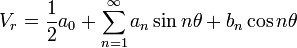
The wind vector field (u,v,w) as a function of altitude above some point (x0,y0) on the surface having an altitude z0 is commonly referred to as the wind profile above that site. Conventionally, it is measured via radio sounding, whereas another approach to this is to use a remote sensing method. Depending on the wavelength of the radiation used, the scattering targets of interest are aerosols (in case of an IR heterodyne Doppler Lidar), air molecules (for an UV Doppler Lidar for observations in clear air, i.e. aerosol free), precipitation (for weather radar), or Bragg Scattering on refractive index variations due to turbulence eddies(for a radar wind profiler). If the respective tracer is moving with the velocity of the surrounding air, the backscattered signal will be shifted in frequency due to the Doppler effect. If this frequency shift is measured, the component of the velocity in the direction of the beam, the radial velocity Vr, is obtained. Using such a methodology, one gets the whole wind profile instantaneously, i.e. not one point at a time like in a radiosonde descent, and with a high update rate.
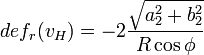
Considering the relationship of the radial component of the wind Vr in the direction of observation
-
 Eq. 1
Eq. 1
with the radar or lidar beam having an elevation angle  and an azimuth angle
  (see figure 3.3.1) , three different directions of observation that are not coplanar are the minimum necessary to determine all three wind components.

3.3.2 Retrieval Algorithms and Errors
A scan strategy widely used by radar wind profilers and vertically pointing Doppler lidars is the Doppler Beam Swinging Technique (DBS), using for example four orthogonal azimuth directions at some elevation close to the vertical and a fifth measurement for the vertical itself. Another technique in this vein has been proposed by Lhermitte and Atlas for precipitation Doppler radars, but of course also applicable to every other dopplerized remote sensing technique, makes use of a full circle scan in azimuth (R.M. Lhermitte, D.A. Atlas, 1961; R.M. Lhermitte 1962). The technique is called Velocity Azimuth Display (VAD), since in the days when fast personal computers were not ubiquitous the horizontal wind and the particle fall velocity were extracted from the actual display of the range gated Doppler shift over azimuth (as an example see figure 3.3.2).

Although the trained observer may be able to extract also characteristics of inhomogeneous wind fields, the general approach would be to fit the parameters u, v and w (w being dominated by the fall velocity of rain drops in the case of weather radar) to Eq.1.
A refined version of the VAD analysis has been proposed by Browning and Wexler (K.A. Browning and R. Wexler, 1968) using more terms of a general Fourier expansion of the VAD graph.
 Eq. 2
Eq. 2
Assuming homogeneous fall speed of rain drops over the area of the VAD circle (or equivalently constant vertical velocity w), the following parameters can be expressed by the first Fourier coefficients (R: radius of the VAD circle). Note that Browning and Wexler used the normal mathematical definition of angles, not the meteorological, and therefore Eq. 5 differs slightly from their publication in that a1 and b1 are interchanged.
- Horizontal divergence:
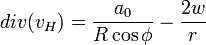 Eq. 3
Eq. 3
- Horizontal wind speed:
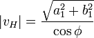 Eq. 4
Eq. 4
- Wind Direction:
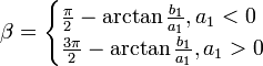 Eq. 5
Eq. 5
- Resultant deformation:
 Eq. 6
Eq. 6
Combining the concept of a linear wind field ( : 3D wind vector,
  : Jacobian matrix)
 Eq. 7
Eq. 7
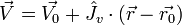
with a full volume scan, Waldteufel and Corbin suggested in 1979 the Volume Velocity Processing (VVP) Method (P. Waldteufel, H. Corbin, 1979) . When Eq. 8 is transformed to polar coordinates (r: Range) and inserted into Eq. 1 setting x0 = y0 = 0 it follows:
 Eq. 8
Eq. 8
Thus, there are a maximum of nine parameters that can be obtained by fitting Eq. 8 to the volume velocity data for each altitude gate. As an example for one of these parameters, a plot of a vertical profile of the horizontal wind is shown in figure 3.3.3. Particularly for the horizontal wind, it is also common to plot wind barbs for each altitude gate. This can be conviently displayed as a time series (figure 3.3.4).


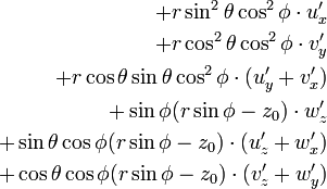
It is worthwhile noting that horizontal vorticity η (the vertical component of the curl of the velocity field, Eq. 9) cannot be extracted, since u'y and v'x only appear summed together.
 ,
,  : unit vector in z-direction. Eq. 9
Since the assumption of a linear variation of the wind field is most likely to hold if the weather situation is stratified, it seems also sensible to set w'x and w'y to zero. Thus, profiles of the following meaningful properties can be obtained by the VVP method in addition to the wind profile: Divergence, vertical shear and Deformation. With regard to sensor synergies, temperature advection as a derived property might be of interest as well. Assuming pure geostrophic wind vg, i.e. the flow of air is devoid of any friction with the surface, gives rise for the following expression (see e.g. Holton 1992)
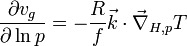 Eq. 10
where T is the thermodynamic temperature, R the gas constant, f the Coriolis factor, and  the horizontal Nabla Operator on isobaric surfaces. Using the ideal gas law, the following relation for the temperature advection holds (Rainbow® 5 instruction manual):
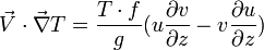 Eq. 11
However, if derivatives of the wind field are to be extracted in addition to the horizontal wind using VVP, one has to be aware that the corresponding matrix used in the fit is generally prone to be ill-conditioned, i.e. the solution varies too strongly with a variation of the arguments with respect to round-off errors due to the finite precision of floating point numbers, or, stated more formally, the condition number C given by the ratio of the largest and the smallest singular value of the matrix XTX encountered in the least square fit procedure is too large, meaning roughly that log10(C) is greater than the machine size precision (for more information see e.g. Wolfram Mathworld). For this reason, Nan et al. have suggested an algorithm called SVVP (S for “stepped”) to overcome this problem (Nan et al., 2007).
3.3.3 Operational performance and technical implementation
The methods presented here are not only different analysis methods, but also imply different scan strategies. Therefore, a trade-off has to be made in order to reconcile update rate, accuracy, representativeness and the possibility to obtain additional information about the nature of the wind field. For weather radars, wind profile quality has been compared by Holleman (Holleman, 2005) for different versions of VAD and the VVP methods. He used two different VAD methods (VAD1: Fourier expansion terminated after the third term, VAD2: Fourier expansion terminated after fifth term) and three different VVP methods with three, six and all nine parameters (VVP1: only wind profile (u0,v0,w0); VVP2: divergence, stretching deformation and shearing deformation in addition to wind profile; VVP3: all parameters from VVP2 along with the vertical derivatives). In fact, only wind profiles obtained from VAD1 have been used for comparison with VVP1 and VVP2, since the single parameters have no effect on each other in value and magnitude of error due to the orthogonality of the basis functions of the expansion and the evenly spaced azimuthal intervals. This is of course not the case for the VVP methods. It must be noted, that the VAD data are not obtained from one azimuth circle, but from the same volume data as the VVP products. The difference is only that in the case of VAD the least square fit has been applied to all azimuth circles individually, whereas for the VVP product the volume data have been subjected to the fit at once. Therefore, the effect of using more data for the VVP than for the VAD is eliminated. During the study data from the KNMI C-band Doppler Weather Radar in DeBilt (Meteor AC360), Radiosonde launches in DeBilt and data from the HIRLAM model (Unden et al. 2002) have been compared for nine months. Products have been generated using the Rainbow® 5 software. The conclusion is that the VVP method is superior to VAD in general. Furthermore, the VVP1 method provides the best horizontal wind values which is attributed to noise fitting due to the non-orthogonality of the basis functions of the fit for VVP2 and VVP3 (and therefore linear dependencies between them). The VVP1 minus background statistics have been found to be at least as good as those of the radiosonde profiles.
3.3.4 Summary and recommendations
Original Contributions Made by EG-CLIMET Action
| Bird echo filter
A Gabor filter has been incorporated in the standard wind profiler software to remove the intermittent echoes due to bird migration. Courtesy, V. Lehmann (DWD). |
 |
| Spectral filtering
Correction of false wind retrievals due to clutter, radio frequency interference and rain events using improved spectral processing which has now been incorporated in the standard wind profiler software. Spurious wind retrievals from the profiler at South Uist on 2 June 2011 are identified by the red boxes. Courtesy, R. Leinweber (DWD) / C. Gaffard (MetOffice). |
 |
| Impact for NWP
It has been demonstrated that strategically placed wind profilers (WP) have a greater impact than radio sondes (RS) in reducing errors in the forecast in the UK (upper) and Germany (lower). The errors are expressed in terms of total dry energy. The analysis used the FSO (Forecast Sensitivity to Observations) technique (Cardinali, 2009) which can identify the contribution to the reduction in the forecast error of specific observations when assimilated into the model. Courtesy, R. Leinweber (DWD) / C. Gaffard (MetOffice). |
  |
Future prospects:
Following EG-CLIMET presentations to EUCOS, the body responsible for the European observing system, E-PROFILE has been launched which will run from 2013-2017 with a kick-off meeting in April-May 2014. E-PROFILE will be responsible for Wind Profiler data quality and for coordinating real time exchange of backscatter profiles from lidars and ceilometers.
The FSO work above has established that Wind Profilers can have a positive effect in improving weather forecasts but only for those instruments where rigorous data quality control procedures have been implemented. FSO has the advantage that it can identify which profilers are performing well and those which are not, and also the advantage of siting wind profilers in data sparse location. E-PROFILE will take this work further.
3.4 Aerosol Backscatter and Extinction profile
The transmission of the atmosphere is highly dependent upon the wavelength of the spectral radiation, and upon the composition and specific optical properties of the constituents in the atmosphere. The prominent spectral features in the atmosphere's transmission spectrum are primarily due to absorption bands and individual absorption lines of the molecular gases in the atmosphere, while a portion of the slowly varying background transmission is due to aerosols.
Recent estimations on the possible impact of aerosols on the radiative forcing (assumed cooling effect) in a global average are of the same order of magnitude as the CO2 effect (warming effect). A full understanding of the role of aerosols is important for improving weather forecasting and understanding climate change. They scatter and absorb both incoming and outgoing radiation (direct effect), and influence cloud formation, their microphysical properties and lifetime (indirect effect). The amount of radiation that is scattered and the directions of scatter, as well as the amount of radiation absorbed, varies with aerosol composition, size, and shape. Thus, the measurements of aerosol optical properties (aerosol backscatter and extinction coefficients at various wavelengths) contribute to the quantification of the radiative forcing, but also to the estimation of particle's physical properties, by inversion of the spectral optical data.
- The backscatter coefficient is a measure of the fraction of incident radiation that is scattered directly back toward the source.
- The extinction coefficient is a measure of attenuation of the light passing through the atmosphere due to the scattering and absorption by atmospheric components (aerosols, molecules). The extinction coefficient is the sum of the absorption coefficient and the scattering coefficient, and generally depends on wavelength and temperature.
Applications: Atmospheric correction for satellite imagery; air quality; health and environment; monitoring of volcanic eruptions and forest fire; Earth radiation budget; radiative transfer models; climate change; aviation safety; visibility.
3.4.1 User requirements and benefits
User requirements and benefits of measuring the backscatter and the extinction coefficient, especially using ground-based remote sensing techniques are described in the WMO's document " Transitioning to operations: lidars and ceilometers" (W. Thomas, DWD, June 2012). Conform to this document: "Atmospheric profiling from ground-based remote sensing instruments has reached a level of maturity making it possible to gather routinely information about the atmospheric state. Recent improvements of data assimilation techniques pave the way for ingesting profile data into models for numerical weather prediction, thus supporting and fostering the operational use of such instruments and measurements. Further applications are long-term monitoring thus climate research at global and regional level and observations of long-range transport phenomena. Current networks are however heterogeneous with respect to the spatial density of instruments, remote sensing capabilities of instruments and products. Consequently, first steps have recently been undertaken to harmonize data and products and to close the gap between research-oriented operations and application-oriented operations."
User requirements refer to data accuracy and data availability. From this point of view, lidars are providing the best accuracy (relative error better than 10%) while lacking continuous operation. On the contrary, ceilometers are all-weather continuous operation instruments, but are lacking the accuracy in retrieving (especially) the extinction profile. Intermediate lidar products are now available with Nitrogen Raman detection capability and have shown a good data availability with a low maintenance thanks to the use of diode-pump lasers. According to Heese et al. (2010), a combination of different instrument types seems feasible as well as appropriate for a prototype aerosol profiling (backscatter and extinction profiles, plus subsequent parameters) near-real-time system that bridges between research-based and operational aerosol observations. The retrieval of first backscatter profiles and secondly extinction profiles (and further mass extinction coefficients) from routine ceilometer measurements is in principal possible, provided that additional measurements are available (sun photometer, advanced Lidars) and that the instrument was calibrated. Note that the conversion of ceilometer data into backscatter and extinction coefficients is associated with large error bars and limited to 4-5 km in daytime conditions. This method is described in Flentje et al. (2010). Elastic backscatter lidars equipped with nitrogen Raman channels are another way to retrieve backscatter and extinction coefficients profiles independently and without assumptions on particle type. As operational lidar products are now available with nitrogen Raman detection capability, these instruments offer an accurate way to self-calibrate the optical extinction profile without any coupling to other sensors. With respect to hazardous aerosol layers (after volcanic outbreaks, dust storms, forest fires) and thanks to continuous monitoring such network may also act as a warning and tracking system of atmospheric particles.
3.4.2 Available techniques
There are several techniques to measure the backscatter coefficient and the extinction coefficient (or at least its integral over a measurement path).
Scattering instruments are used to measure a basic optical property of the air sample: the volume scattering function. Scattering instruments include integrating nephelometers, backscatter meters, forwardscatter meters, and polar nephelometers. Integrating nephelometers perform a point measurement of the light scattered over a range of angles and permit determination of the scattering component of extinction. The air sampled by the integrating nephelometer is enclosed and illuminated indirectly by an artificial light source, allowing automated continuous day and night operation. Nephelometers have been used in a variety of applications (Charlson et al., 1978). Since nephelometers involve point measurements, care must be taken to minimize the influence from local sources. Also, inhomogeneous impairment, such as plume blight, cannot be detected.
Photometers measure light intensity using a photodetector, which converts brightness into representative electric signals. By the use of combinations of lenses and filters, different optical properties may be determined. Sun photometers are photometers pointing at the Sun. Recent sun photometers are automated instruments incorporating a Sun-tracking unit, an appropriate optical system, a spectrally filtering device, a photodetector, and a data acquisition system. These instruments measure the solar radiance after the absorption / scattering from the atmosphere, at several wavelengths. The integral of the extinction coefficient (AOD), as well as other column optical and microphysical parameters can be extracted from multiwavelength sun photometer data.
Transmissometers are instruments which measure the amount of light transmitted from a specified source (artificial) to a receiver, allowing the direct calculation of the average extinction coefficient of the air along the instrument path. When transmissometers are used in very clean atmospheres, their critical sensitivity to atmospheric turbulence can introduce error. Additionally, these instruments are usually limited to a single wavelength and not very portable.
Lidar provides a method of directly measuring the optical properties of atmospheric aerosol distributions, as well as of other atmospheric parameters or components (molecules and fluorescent species, wind velocity and direction, temperature and water vapor) as profiles. Lidar makes use of a laser to excite backscattering in the atmosphere. This backscattered signal is observed using a telescope receiver, which collects the light and send it to the receiver optics. The role of the optical chain is to select specific wavelengths, split between them and direct them to photodetectors, which further convert the optical signal into electrical signals. These are recorded as a function of time by analog-to-digital converters and/or photon counting devices. Each lidar signal represents, therefore, the spatial variation of the measured parameter, i.e. the vertical, slant or horizontal profile of the variable.
Interaction of the laser beam with the atmosphere is complex. Multiple phenomena are produced simultaneously, both elastic (i.e. at the same wavelength: Mie and Rayleigh scattering) and inelastic (i.e. at a different wavelength: vibrational and rotational Raman, fluorescence). Thereby, the set-up of the lidar is application-driven. The backscatter coefficient can be measured using simple elastic backscatter lidars and several types of ceilometers, although some assumptions has to be made (see the "Retrieval algorithms and errors" sub-section). For the measurement of the extinction coefficient, inelastic (vibrational or rotational) Raman detection is generally used. The combination of the two gives independent estimation of both parameters. High Spectral Resolution Lidars take advantage of the spectral distribution of the lidar return signal to discriminate aerosol and molecular signals and thereby measure aerosol extinction and backscatter independently. Multi-wavelength detection is also recommended in order to extract supplementary information (e.g. intensive optical parameters such as Angstrom exponent, color indexes and color ratios, or microphysical properties such as size distribution, complex refractive index and single scattering albedo.
| Table 3.4.1: Advantages and limitations of the various aerosol lidar types | |||
|---|---|---|---|
| Lidar type | Principle | Retrieved parameters | Limitations |
| General |
|
|
|
| Ceilometers |
|
|
|
| Elastic backscatter |
|
|
|
| Elastic backscatter and Raman (vibrational / rotational) |
|
|
|
| Multi-wavelength Raman |
|
|
|
| High Spectral Resolution |
|
|
|
Lidars provide important advantages in the determination of the backscatter and extinction coefficients: high spatial resolution (1 value each 3 - 60 m), high temporal resolution (1 profile each 1 - 60 min), high dynamic range (0.2 ... 15 km). There are two important types of errors associated to the measurement of the backscatter and extinction coefficients from lidar: a) instrumental errors due to technological limitations (both at components' level and their integration); b) retrieval errors due to the non-determination of the lidar equation (not exhaustive, see Section "Retrieval algorithms and errors"). Nevertheless, the quality assurance program developed by the European Aerosol Research LIdar NETwork EARLINET made possible the estimation of the backscatter and extinction profiles with an uncertainty less than 10%, which is proper for microphysical inversion and climatological studies. The range in which this uncertainty threshold is kept depends on the individual lidar systems (the signal-to-noise ratio of the channels).
3.4.3 Retrieval algorithms and errors
Whatever the set-up of the lidar system, the magnitude of the received lidar signal is proportional to the number density of the atmospheric diffusers (molecules or aerosols), their intrinsic properties (i.e. probability of interaction with the electromagnetic radiation at the laser wavelengths, called cross–section value) and with the laser incident energy (Measures, 1992). Therefore, obtaining information about the aerosols means to find solutions of the equation which relates the characteristics of the received and emitted signal, and the propagation medium. The form of the equation depends of the interaction type. The basic lidar equation takes into account all forms of scattering and can be used to calculate the signal strength for all types of lidar, except those that employ coherent detection. The propagation of light in an inhomogeneous medium is well described by the electromagnetic theory.
The detected light backscatter power at the wavelength λD from a distance R can be expressed as follows (Nicolae, 2010):
where RCS is the range corrected signal of the lidar and Cs is the instrument function.
The atmospheric backscatter coefficient ![]() is a key element of the lidar equation, and is proportional to the cross section of the involved physical process and to the number density of the atmospheric active diffusers (i.e. atoms, molecules, particles, clouds) in the probed volume.
is a key element of the lidar equation, and is proportional to the cross section of the involved physical process and to the number density of the atmospheric active diffusers (i.e. atoms, molecules, particles, clouds) in the probed volume.
The atmospheric transmittance from the transmitter to the probed volume and from the probed volume to the receiver, respectively, are expressed as the integrals of the atmospheric extinction coefficient and may be different on the two directions of the laser pulses, as is the case of the Raman backscatter radiation (λD = λR ≠ λL). The atmospheric extinction coefficient, backscatter coefficient and the backscatter cross section refer to all possible physical interactions within the atmosphere.
Both in case of elastic backscatter lidar, and Raman lidar, the solution of the equation is not unique (Kovalev,2004), since it has two unknowns: backscatter and extinction coefficients. Combination of elastic and (vibrational) Raman channels allow to retrieve these parameters with minimum assumptions:

where the “L” and “R” indexes correspond to laser and Raman detected wavelength, respectively, and k ranges between 0 for coarse mode particles (maritime, dusts) and 1.5-2 for fine mode particles (pollution forest fires). This relation is valid if the difference between the Raman and laser wavelength is small. Nitrogen molecules are used to obtain the Raman signal, due to the fact that Nitrogen is considered a gas with constant concentration over time and has a Raman spectra easy to be separated from the Rayleigh one. In this case, the second (532 nm) and third harmonics (355 nm) of Nd:YAG laser can be used as excitation, since the associated Raman lines are close to these wavelengths: 607 nm and 387 nm, respectively. With this hypothesis, the aerosol extinction coefficient at the laser wavelength can be obtained by applying the natural logarithm and the derivative to the Raman lidar equation.
Molecular parameters (indices "m") can be calculated with sufficient accuracy from ground values of pressure and temperature using an atmospheric model, or radiosounding. A simple mathematical procedure applied to the couple elastic + Raman channel leads further to the retrieval of the backscatter coefficient (Mattis, 2002). With different couples of elastic and Raman channels, extinction and backscatter coefficients at several wavelengths can be computed, and therefore more products can be obtained (Müller,1999a): lidar ratios, Angstrom exponents, color ratios and even microphysical parameters such as size distribution, effective radius, complex refractive index, single scattering albedo, volume and number concentration.
Two kinds of errors are associated to the retrieval of the backscatter and extinction from lidar measurements: statistical errors and systematic errors.
1. Statistical errors are mainly due to the to signal detection, i.e. background of sky and dark current of detector (Theopold and Bösenberg, 1988). Directly related to this kind of error, there is the error introduced by operational procedures such as signal averaging during varying atmospheric extinction and scattering conditions (Ansmann et al., 1992; Bösenberg, 1998). Statistical errors can be assessed either by analytical propagation (Gaussian or Poison statistical distributions have to be considered), either by Monte Carlo techniques.
2. Systematic errors generally arise from:
a) the estimation of temperature and pressure profiles (Ansmann et al., 1992);
b) the estimation of the ozone profiles in the UV (Ansmann et al., 1992) and in other spectral ranges;
c) the wavelength dependence parameter k (Ansmann et al., 1992; Whiteman, 2000);
d) the multiple scattering (Ansmann et al., 1992; Wandinger, 1998; Whiteman, 2000);
e) the overlap function (Wandinger and Ansmann, 2002).
Systematic errors are more difficult to estimate and this is still an open scientific issue.
3.4.4 Operational performance and technical implementation
Although lidar technique has been used for many years, recent technological developments, coupled with the implementation of modern mathematical procedures have led to a more operative use of lidar systems. Ceilometers are nowadays more and more complex and sensitive, some new products being able to detect aerosols and therefore to deliver the backscatter coefficient with the coupling of other sensors and with a large error (more than 50%). On the other hand, powerful lidars are more and more automatic and suitable for a 24/7 unmanned operation. Elastic lidars equipped with nitrogen Raman detection channel are intermediate solutions for an accurate self-calibration and an independent retrieval of backscatter and extinction coefficient profiles without any coupling to other sensors. New industrial and operational nitrogen raman lidars based on diode-pump lasers have shown a low maintenance and a high data availability. The main progresses recorded in the last years are referring to the improvement of the instruments and retrieval algorithms for:
1. the automation of the operation
From an operational point of view, alignment of the laser beam into the receiver FOV is critical. Depending on the configuration, the overlap control needs to be very precise (order of 0.01 mrad) and stable with temperature. Short term fluctuations in the laser energy are usually averaged out during the integration time of the measurement. However, long term drift in the laser energy is important if the lidar is to be kept running for longer periods of time. Therefore, laser energy should be at least monitored and eventually stabilized. In case harmonics of the fundamental laser frequency are used, conversion crystals are used (SHG, THG) that alter the direction of the outgoing laser beam when they are tuned. This has to be compensated for in order to keep the overlap properly aligned. If the (generally non-eye safe) lidar is to be kept running for longer periods of time, in particular if the operator is not present from time to time, safety precautions have to be taken according to proper use of lasers outdoors. Remote control of the lidar operation (e.g. via web tools) is an option.
2. the improvement of the dynamic range
Telescopes with large apertures for high troposphere and stratosphere exploration tend to have large focal lengths, which tends to reduce field of view and increase the distance at which field full overlap is reached. To overcome this problem, two receiver sets, using different telescopes (one for far range, another, with smaller aperture, shorter focal length and nearer full overlap distance, for close range), can be used. Other solutions based on specific optical components are also available in order to reduce the overlap and ensure the highest range as possible.
Measurements can also be corrected under the full overlap height if the overlap function of the system has been measured.
Increased dynamic range can be achieved also with combined analog and photoncounting techniques.
3. the improvement of the temporal coverage
Daytime performance of (vibrational) aerosol Raman lidar can be achieved by sufficiently suppressing the daytime background and/or by increasing the emitter power. Narrowing down interference filter passband has consequences for the optical design of the receiver (angular dependence of the position of the passband transmission peak). Other solutions exist, e.g. grating/monochromators, tilt slit diaphragm. The limited acceptance angle of small bandwidth interference filters IFF determines the whole lidar optics design.
Ceilometer detection and inversion capabilities are also limited to the lowest part of the troposphere (up to 4-5 km) in daytime conditions.
4. reducing the uncertainties of the final products
The minimum recommendation for an optimized product is to add a nitrogen Raman channel to a backscatter lidar, so that both the backscatter and the extinction coefficient can be derived independently. The same can be achieved by using a HSRL system and / or a scanning lidar (multiple zenith-angle measurements). This latter technic requires a strong assumption on horizontal and temporal stability of the atmosphere. Moreover their use in operational networks has to be demonstrated. The implementation of state-of-the-art algorithms and tools for the correction of the signal as well as for the inversion of the corrected signal contributes both to reducing the uncertainties and to increasing the availability of the data. This includes:
- signal pre-processing: cloud screening, pile-up correction, estimation of the statistical error, background subtraction, range correction, handling of signals measured at angle different from zenith, correction for depolarization-dependent receiver transmission, calculation of the profile of the Rayleigh-scattering coefficient, correction for Rayleigh-transmission, temporal averaging to create fixed time intervals, vertical smoothing up to a fixed height resolution
- calculation of the extinction coefficient from the Raman signal: calculation of the derivative, estimation of the uncertainty of the derived extinction, determination of the overlap function
- calculation of the backscatter coefficient from combined elastic - Raman signals: detection of the reference height, estimation of the reference value
Significant improvements can be achieved by the automation of the lidar inversion, to avoid human error and operator subjectivity.
3.4.5 Summary and recommendations
Although satellite imagery (with its increasing temporal and spatial resolution) and satellite remote sensing will ensure in the future the growing need for knowledge of global optical properties of the atmosphere, accurate estimation of the aerosol backscatter and extinction coefficients, especially near ground and in the first atmospheric layers, can be only provided by ground-based remote sensors. Laser-based techniques have the main advantage of high spatial and temporal resolution. Two solutions can be retained for improving short-term weather forecasts and climate change trends analysis, as well as warning and tracking system of atmospheric particles:
- Firstly, a network of operational lidars equipped with depolarization and nitrogen Raman detection channels are the solution for an accurate self-calibration and an independent retrieval of backscatter and extinction coefficient profiles, as well as the ability to classify the aerosols.
- Secondly, a network of ceilometers, backed-up by multiwavelength Raman lidars and sun photometers, can be an alternative but where the operational use (24/7) of multi wavelength lidars has not been widely demonstrated and where the real capacity of ceilometers to measure above 5 km is not ensured.
Nevertheless, current networks are however heterogeneous with respect to the spatial density of instruments, remote sensing capabilities of instruments and products.
In this respect EG-CLIMET recommends the following:
1. European and national funding agencies should invest more in the technological development of:
- Nitrogen Raman lidars with depolarisation - continuous (i.e. daytime), unattended operation
- ceilometers - multiwavelength capabilities, increasing dynamic range, increasing the signal-to-noise ratio
- network infrastructure, storage capacity and software development, in order to build up the capacity for enhanced usage of profiling instruments
2. European research (EARLINET/ACTRIS) and operational networks (NMHSs, UK Met. Office, DMI, DWD, FMI, KNMI, Meteo-France, SMHI etc.) should develop an optimized and fully automatically working method for a network of different instruments. They should set up working groups to:
- encourage and support the set-up of measurement stations with parallel operations of ceilometers, lidars and sun photometers
- harmonize lidar / ceilometer observations and data products/data formats
- organize and support intercomparison campaigns for ceilometers and Lidars (involvement of EARLINET[/ACTRIS recommended)
- define best practices for ceilometer calibration (self-calibration technique, cross-calibration with Lidars and sun photometers), quality assurance, and long-term operations
- define a common data format for data exchange/data storage at scientific level and at operational (national weather services) level, including data policy
- take advantage of existing algorithms and implement homogeneous automatic data processing procedures in order to increase the near-real-time capability of the networks
- integrate European national ceilometer networks and lidar networks into GAW Aerosol Lidar Observation Network GALION, for global coverage
3. GMES “Atmosphere Core Service” initiatives (e.g. MACC II) together with European lidar and ceilometer networks should push for the use of ground-based remote sensing data for:
- validating aerosol parameters of the global integrated (chemistry + dynamics) C-IFS model operated at ECMWF
- contributing to regional models at higher spatial resolution
- assimilating aerosol profiles into models and validation strategies
4. European lidar and ceilometer networks together with WMO, various expert groups (e.g. EG-CLIMET, CIMO, CBS, WEZARD) and national and international aviation control institutions (e.g. EASA, Eurocontrol, ICAO) should set up working groups to:
- support long-term monitoring of aerosol parameters/aerosol profiles
- set up tools to make the current instrumental network available to users
- organize data exchange procedures and data policy
- close the gap between research-oriented operations and application-oriented operations (weather and climate, aviation safety, air quality)
3.5 Target classification
3.5.1 Introduction
The core instrumentation for clouds and aerosols quality controlled-observations comprises:
- Lidar/ceilometer providing profiles of
- attenuated backscatter coefficient from aerosol and cloud
- linear depolarisation ratio
- Doppler cloud radar operating at 35 or 94GHz, providing profiles of
- reflectivity, Z,
- mean Doppler velocity, v,
- Doppler spectral width, σv,
- standard deviation of the mean Doppler width, σvbar
- linear depolarisation ratio, LDR.
- Microwave radiometer providing
- brightness temperatures at two or more wavelengths in the range 20-30 GHz
- derived water vapour and liquid water path
- Additional observations
- surface rain rate from raingauge
- radiosonde profiles, or NWP model output (temperature, pressure, humidity, winds)
The profile of attenuated backscatter coefficient, from a lidar/ceilometer, exhibits returns from aerosol, ice and liquid. The molecular return may also be present at visible lidar wavelengths. Attenuation by liquid is severe, and the lidar signal does not penetrate liquid layers that are deeper than about 300 m, thus only reliably detecting the cloud base. Penetration through ice clouds can reach 3 km or more. The lidar depolarisation ratio potentially provides information on the shape and type of particles responsible for the lidar return. The cloud radar is sensitive to precipitation, ice, snow, insects and liquid droplets.The cloud radar is much less affected by attenuation and provides profiles of the first three moments of the Doppler spectra; reflectivity, Z; Doppler velocity; and the spread of Doppler velocities. Additionally, the variation of the mean Doppler velocity can also be calculated; this can be used for estimating the turbulent properties of the atmospheric particulate, or highlighting the random motion displayed by an insect. The linear depolarisation ratio, if available, is useful for distinguishing insects from clouds and precipitation within the boundary layer, and for identifying the location of melting ice particles.
3.5.2 Input datasets
The essential instruments that must be present are vertically pointing cloud radar and backscatter lidar, together with either regular radiosonde profiles, or hourly model forecast data available over the site. Recommended but non-essential instruments are microwave radiometer (for providing liquid water path) and rain gauge. Processing is done one day at a time. Ideally the instruments operate continuously, but if at any time in the day radar, lidar or model data are missing then there will be a gap in the output product. The absence of data from the non-essential instruments may mean that correction for radar attenuation is not possible, but data quality flags will indicate that this is the case.
The decision regarding which instruments and auxiliary data to include in this product was made by considering those that are most used in retrieval algorithms and those that are necessary to correct for radar attenuation and flag bad data. Radar and lidar are complementary due to their very different dependence on particle size; this means that the combination of the two offers the most accurate estimates of cloud occurrence and cloud fraction (Mace et al. 1998, Hogan et al. 2001), and can also be used to retrieve particle size (Donovan et al. 2001, O’Connor et al. 2004). However, it is not the intention that all instruments at a site that could conceivably be used in a retrieval algorithm (or that might be useful for model comparison, such as broadband fluxes) should be combined into this product; instead, routines for placing other instrument data on the same time-height grid are provided for this task.
The algorithm is implemented in Matlab, although future implementation in C and/or python is possible. The input datasets are read into the processing algorithm using separate functions that may make modifications depending on the particular instrument and site.
3.5.3 Cloud radar
The vertically pointing radar would typically operate continuously at 35 or 94 GHz and provides profile with a time resolution of around 10-30 seconds and a height resolution of 30-60 m (better than 100 m). The radar resolution is used as a master grid on to which all other datasets are placed. The temporal resolution of 30 s is long enough that the datasets are conveniently small to use, but short enough that cloud fraction and other parameters to be used to evaluate models are of sufficiently high precision. Essential parameters that the radar must provide are radar reflectivity factor Z and Doppler velocity ν (There are some sites with current and/or legacy data without Doppler velocity; the algorithm may be modified in future to cope without Doppler velocity). Radar reflectivity factor should have had the following processing applied to it:
- Linear averaging to the resolution required.
- Noise subtraction: the reported Z should be that of the atmospheric targets without the contribution from instrument noise and thermal emission that is present in the raw measurements.
- Clear sky clearing: areas with no detectable atmospheric signal should be flagged (or SNR should be available). Any remaining speckle noise should be removed using masking algorithms.
- Elimination of artefacts, such as the near field effect for instruments with large antennas, overlap effects for some bistatic systems and spurious instrument-specific echos.
Note: Although definitions and processing may be performed with Z in linear units, it is conventional to report the values in logarithmic dBZ units defined thus:
![Z [dBZ] = 10 \log_{10} Z [mm^6 m^3]](/wiki.eg-climet.org/images/math/8/7/4/8749629620b394336bccb54a76c7502a.png)
The quality control algorithm attempts to flag likely ground clutter, but since the clutter behaviour can be very different for different radars it is better if it can be removed prior to being read in. Likewise, it is beneficial but not necessary for insects to have been identified; if available, the LDR parameter is an excellent discriminator. The radar should report values as low as possible above the ground. No attempt should be made to correct for attenuation. The radar should obviously be calibrated as well as possible and an indication of the likely accuracy of the calibration should be available. If necessary the appropriate factor will be applied to Z in order to conform to the following calibration convention, defined for a distribution of Rayleigh-scattering liquid water droplets in the absence of attenuation:
in the absence of attenuation, a cloud at 0 °C containing one million 100 μm (i.e. Rayleigh scattering) droplets per cubic metre will have a reflectivity of 0 dBZ at all frequencies.
If several reflectivity channels are available from a particular site, such as the four specialized modes used by the MMCR radars on the ARM sites (Clothiaux et al. 1999), then the one most free from artefacts will be taken, even if this is not the most sensitive. This is because the Instrument Synergy/Target Categorization product is intended to be used in automated algorithms that operate on large volumes of data without the need for significant human quality control. The Doppler velocity should have had clear sky pixels removed in the same way as Z. If necessary, the values will be inverted to ensure that the convention of positive velocities upwards is adhered to. The velocities need not be unfolded, but the folding velocity νfold should be known to the algorithm. It is possible that the algorithm for locating the melting layer (see section 3.4.1) will perform poorly if the folding velocity is too small.
Other radar parameters, such as spectral width ( ), will be transferred into the output dataset. If available, the 30-s standard deviation of the 1-s mean velocities,
  (used to estimate turbulence levels; Bouniol et al. 2003), will be used to assist in the diagnosis of ground clutter.
3.5.4 Cloud lidar
The cloud lidar is principally used to identify the base of liquid water clouds. Most commonly this instrument will be a ultra-violet, visible or near-infrared lidar ceilometer reporting only attenuated backscatter coefficient, β. The instrument should be operated pointing between 2 and 5 degrees from zenith to avoid specular reflection from horizontally aligned pristine crystals, which could be mistaken by the algorithm for the presence of supercooled liquid water (Hogan et al. 2003b). The lidar should be calibrated as well as possible (e.g. using the technique of O’Connor et al. 2004). Units are in m-1 sr-1. Two algorithms are proposed here:
1. The CLOUDNET algorithm assumes that all signals from the lidar are due to atmospheric particulates such as cloud and aerosol, rather than Rayleigh scattering from air molecules. This is generally valid in the near infrared (e.g. 905 nm used by the Vaisala CT25K and CT75K instruments) but for lidars at visible wavelengths (e.g. 532 nm micropulse lidars used by ARM), an additional processing step is necessary to identify and flag the molecular return. Background and solar noise should also be identified and flagged in the pre-processing step.
2. The STRAT algorithm (Morille et al. 2007) performs a target classification based on total attenuated backscatter Lidar data. STRAT identifies in each Lidar profile the following categories: (1) portion of the profile where signal-to-noise ratio is below a given threshold, (2) portion of the profile likely to be particle-free (molecular backscatter), (3) portion of the profile with aerosols or clouds (aerosol/cloud separation is available), (4) portion of the profile corresponding to the mixing layer. A configuration file must be adjusted to help optimize the performance of STRAT. STRAT operates on a single Lidar channel, but can be used for any wavelength (ultra-violet, visible or near-infrared). STRAT is developed under GPL licence and available for download at STRAT software download
Note that lidars with Raman or depolarisation channels are far superior in their discrimination between the various atmospheric particulates; the depolarisation ratio and the extinction are extremely useful parameters for liquid water diagnosis and cloud retrievals, and these are provided in the Instrument Synergy/Target Categorization for instruments in quasi-continual operation.
3.5.5 Model parameters
At least four radiosonde profiles per day would be required from close to the site to provide adequate dynamic and thermodynamic data above the instruments. Because most sites do not have this information, we use hourly profiles from short-range model forecasts. These models assimilate the data from the radiosonde network so the temperature (T), pressure (p), humidity (q) and horizontal wind (u and v) will usually be accurate enough for our purposes. We do not make use of the cloud variables as these are to be evaluated, and will generally be much less accurate. Before it can be used the model output must be converted into the Cloudnet single-site model format, which includes calculation of a number of radar propagation and scattering parameters at 35 GHz and 94 GHz that depend on thermodynamic state. The variables T, p, u and v are then interpolated on to the time grid of the radar and provided as part of the Instrument Synergy/Target Categorization product. To conserve space, they are not interpolated in height; subsequent processing algorithms will need to do this. The following additional parameters are ingested and used by the algorithm: specific gas attenuation kg (dB km-1) (predicted from model q, T and p using the line-by-line model of Liebe 1985), specific gas attenuation for saturation with respect to liquid water kgs (dB km-1) and specific liquid water attenuation kl (dB km-1 [g m3]-1), using the formulation given by Liebe et al. (1989).
3.5.6 Microwave radiometer
A recommended but optional input dataset is liquid water path (LWP) derived from dual- or multi-frequency microwave radiometers. LWP is used in many retrieval algorithms for liquid water clouds. Ideally LWP will not be derived using climatologically tuned coefficients, as these can result in errors exceeding 50 g m-1 and retrieved values that are negative. One method is described by Gaussiat (2004) which makes use of other sources of data to provide more accurate coefficients; lidar is used to locate the height (and therefore the temperature) of liquid cloud, and the model to provide a more appropriate humidity distribution than climatology. Also, profiles identified by the lidar to be free of liquid water cloud are used to estimate the zero offset and by interpolation across periods of cloud, to provide considerably more accurate LWP in thin cloud. This approach also has the advantage that it can produce accurate LWP even if with poorly calibrated radiometer channels. LWP is important for the correction of radar attenuation in liquid water clouds; at 94 GHz it can exceed 5 dB and so if correction is not performed then reliable retrievals in ice clouds above liquid clouds based on the value of Z are impossible.
3.5.7 Rain gauge
The presence of rain on the dish or radome of a radar can result in a large and variable attenuation (Hogan et al. 2003a), of order 10 dB, making it impossible to use the absolute value of Z with any reliability. Rain itself also extinguishes the signal and can be difficult to correct for; microwave radiometers do not provide accurate LWP estimates in rain (Crewell and Loehnert, 2003). Radar attenuation due to the melting level is also uncertain. To diagnose the presence of rain we use either a rain gauge or the radar itself. Ideally the rain gauge should have a fairly high sensitivity; tipping-bucket gauges in particular can be very slow to register the start of light rain events. The radar parameters Z, v, and in the lowest few gates can also be used to diagnose probable rain on the ground. This approach tends to be more sensitive than a rain gauge, so the rain gauge is not treated as an essential input dataset.
Further technical details on the algorithms can be found at Cloudnet home page.
3.6 Mixing height
3.6.1 Fundamentals
The mixing layer height (MLH) is the height of the layer adjacent to the ground over which pollutants emitted within this layer or entrained into it become vertically dispersed by convection or mechanical turbulence within a time scale of about one hour (Seibert et al., 2000). As shown in Figure 3.6.1, during daytime the mixing layer tends to be unstable as a result of convection and is capped by an entrainment zone. At night a shallow stable layer forms near the surface in which mixing occurs through intermittent turbulence, leaving a residual layer above.

MLH is an important parameter for practically all air pollution applications except probably the street scale; it is still one major uncertainty for most air quality models. Different instrumentation and different parameterizations will give variable estimates of MLH. Most desired for air pollution applications are continuous representative time series of MLH for the site of interest. As this is still difficult to achieve with routinely available instrumentation e.g. from NWS networks, also simple parameterizations or even fixed or prescribed values (day/night-time, eventually dependant on atmospheric stability) are still in use. Whereas in convective conditions, MLH is often – and rather straightforward - determined as the capping lid (elevated inversion base) of the convective boundary layer, there is more debate on how MLH is best determined in night-time stable conditions, and which physical processes are relevant for MLH evolution at night.
As pointed out in Seibert et al. (2000), there is no ‘MLH-meters’ able to determine the MLH without uncertainties and assumptions. Furthermore, the definitions itself of Mixing Layer are dependent on the quantity employed in the definition itself. Being the mixing due to turbulence, the best definitions appear those making use of the turbulence. Unfortunately, direct measurements of turbulence are very complex, and its remote sensing is currently out of our reach. As a surrogate, we can alternatively measure some proxies or drivers of the turbulence, as the temperature and wind profile, the energy fluxes, the profile of pollutants. The remote sensing of these parameters has become now possible with a variety of instruments, and the evaluation of the MLH is then possible as well. However, some assumptions may be made according to the technique employed. For example, the potential temperature is used in the parcel method and related techniques (all those using the temperature profile). However, this makes sense only under convective regimes, being the potential temperature profile a proxy of convection. Mechanically-induced turbulence cannot be determined by this approach. Likewise, the aerosol can be used as a tracer of the mixing processes in the PBL, even though advection from long distances may complicate the scenario and make very difficult the tracking of the MLH, especially by automated algorithms. This problem lead to attribution problems that will be discussed later on. In case of stable boundary layer, in fact, some problems limit the applicability of remote sensing techniques to determine the MLH. One is related to the minimum altitude of reliable detection, different for each instrument and dependant on the sounding technique (sodars and mini-sodars allow the first gate to be within a few meters, while electromagnetic-related techniques usually suffer for a larger blind zone).

On the other hand, the definition itself of stable boundary layer is complicated by the fact that the turbulence in the stable boundary layer is rather complex, and however weak. The SBL is usually represented as composed by two layers: the lowest, in contact with the soil, showing mostly continuous turbulence, caused by wind shear and radiative forcing. The upper layer is characterized by sporadic turbulence, caused mainly by breaking of gravity waves, presence of clouds and wind shear. Since the profiles are usually smooth, a good quantity for comparisons is the Integral Scale Depth of SBL, as proposed by Stull:
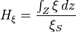
Where ξ can be potential temperature, relative humidity or any other quantity with asymptotic behavior towards the free troposphere. This means that it is often very hard to compare MLH measurements if based on different instruments or different proxies (adapted from Stull).
3.6.2 Available Techniques
Mixing layer depth can be determined either (1) using temperature, humidity, wind and turbulence profiles from in-situ or remote sensing based vertical profiles or (2) by tracing gradients in atmospheric constituents or structures using remotely sensed vertical profiles (lidar, wind profiling radar, sodar). This is illustrated in Figure 3.6.3. It is important to keep in mind that the (dis)agreement between different retrievals (e.g. temperature based vs aerosol based) is driven to a large extent by the (in)consistency between the atmospheric parameters of interest (e.g. potential temperature profile vs aerosol concentration profile).

Techniques to derive the mixing layer depth (MLD) from thermodynamic vertical profiles date back to the 1970’s. Extensive reviews are published on this topic regularly. Similarly methods to diagnostic MLD from model or analyses fields are also well described in the literature. An overview on methods how to derive MLH from measurements as well as parameterizations in meteorological pre-processors are given in Fisher et al. (1998; COST action 710). A paper by Seibert et al. (2000) provides a review and intercomparison of operational methods for the determination of the mixing height. A review of methods for urban areas is given in Piringer and Joffre (2005; COST action 715). Emeis et al. (2008) provides a review of surface-based remote sensing of the mixing-layer height. The reports reflect the status of MLH retrieval shortly before they were finalized.
The table 3.6.1 summarizes tracers and instruments that can be used to estimate the depth of the mixing layer. Without being fully comprehensive, it provides a quick overview.
| Table 3.6.1: Tracers and instruments used to estimate the depth of the mixing layer | |||
|---|---|---|---|
| Tracer | Instrument | Pros | Cons |
| Temperature |
|
|
|
|
|
| |
|
| ||
|
|
| |
|
|
| |
| Vertical wind |
|
|
|
|
|
| |
|
| ||
|
|
| |
| Aerosol |
|
|
|
|
|
| |
|
|
| |
| WV |
|
|
|
|
|
| |
|
|
| |
|
|
| |
| Radon |
|
|
|
| Turbulence |
|
|
|
From lidars and ceilometers, the MLH may be derived using different proxies, according to the measured parameter:
Rayleigh (elastic) lidar
Provides the aerosol backscatter profile, and the MH is hence based on the assumption that ground-emitted pollutants (like the aerosol) is dispersed and mixed within the whole PBL by turbulence. Three different techniques have been proposed for the MLH determination from aerosol backscatter profiles and will be discussed in sect. (YY).
Raman (water) lidar
The Raman lidar may provide the water vapor mixing ratio profile, if the suitable channel is operating. The water vapor profile may be employed as the aerosol profile, if it can be assumed produced at ground and mixed by atmospheric turbulence.
Doppler (wind) lidar
Doppler lidars provide the profile of wind (u, v, w), making it a very promising instrument for the detection of turbulence (if suitable spatial-temporal resolution is achieved), and convection through the w component. These quantities are directly connected to the turbulence processes and this kind of instrument can then provide a reliable information about the PBL dynamics. However, these instruments are still expensive and have not reached a large diffusion yet. Moreover, the commercial wind lidars make use of the aerosol signal (which is orders of magnitude larger than the molecular one), so the presence of aerosol is, again, mandatory for a good signal-to-noise ratio and the determination of the MLH.
3.6.3 Retrieval algorithms based on aerosol backscatter Lidars and ceilometers
As mentioned in sect. 3.6.2, the determination of the MLH by lidar/ceilometers consists in solving two different problems: first, the recognition of all the aerosol layers, and then the attribution of the PBL top to one of the layers found. This problem is sometimes referred to the ‘attribution problem’, and will be presented in section 3.6.4. Here the problem of the layer recognition will be discussed.
Almost all operational eye-safe lidars (historically known as ceilometers) make use of Rayleigh scattering to provide information about clouds and aerosols throughout the troposphere. The Rayleigh echo from molecules and aerosols allow the elastic lidars to measure the aerosol backscatter coefficient, and, with greater uncertainty, the extinction coefficient and the optical thickness. So far, the calculation of these products requires attended calibration of the instrument and data inversion, although several semi-automated methods have been proposed so far (O’ Connor; Wiegner and Geiss). This aspect is described in sec. 3.4. However, this is a rather time-consuming activity, and hence it is not suitable for continuous and operational observations.
In the recent years, several techniques have been investigated to automatically derive some useful information from raw lidar profiles. These information include: cloud base (and eventually top), cloud coverage, presence of rain, and height of the mixing layer. This latter, in particular, is still an open task since several problems still limit the reliability of such product.
However, several automatic analysis may be performed using the background-subtracted signal coming from the instrument, eventually under the form of Range-Corrected Signal (commonly referred to as RCS or Pr2) or logarithm of RCS. The determination of aerosol layers is usually performed on the RCS or ln(RCS), although some authors prefer the signal.
The methods proposed so far to infer the boundary layer height, also referred to as mixing layer height or mixing height, from elastic lidar backscatter data may be classified in three categories:
- threshold method;
- variance method;
- gradient method.
The threshold method has been proposed by Melfi et al. (1985), and is based on the assumption that the aerosol load in the free troposphere is very low. In this case, the aerosol backscatter is significantly higher than zero only in the PBL. The ML is then determined as the zone, close to the ground, where the backscattering exceeds a fixed threshold. This technique requires a good signal-to-noise ratio, being quite sensitive to noise in the data.
The variance method is a powerful technique that employs the temporal variance of the signal to detect the MH (illustrated in Figure 3.6.4). In fact, it has been shown that a maximum in the aerosol backscatter signal is associated to the entrainment zone, which is the interface between the mixed layer and the free troposphere. This layer is characterized by the different eddies reaching different heights, causing a large variance in the aerosol cross section.


However, although this method is very powerful for the determination of the convective boundary layer, its reliability under stable or neutral conditions has not been proved so far. When turbulence is very weak, as often happens during nighttime, not necessarily the highest variance is directly connected to the top of the mixing layer. In these conditions is even hard to define the mixing layer, and often the most reliable method to detect the mixing status of the atmosphere is a direct measurement of the aerosol distribution (Seibert et al, 2000). However, the use of variance to detect the height of the stable boundary layer has been further investigated by Pal et al. (2013, submitted). Another key point concerning the variance method is that it requires a very high signal-to-noise ratio, so that the variance can be attributed to variation in the signal and not induced by noise. Many ceilometers, especially those composing current networks are not powerful enough to provide a reliable variance profile with acceptable time resolution. Next generation ceilometers will likely allow to use this quantity to add valuable information to the MLH determination procedures.
The gradient method has been proposed by Endlich et al. (1979), and rests on the hypothesis that the aerosol is produced at ground and is well mixed within the boundary layer. The lowest inflection point detected in the aerosol backscatter coefficient indicates the MLH. The identification of the inflection points can be performed either by direct numerical differentiation (the first (a) or second (b) derivative of the range-corrected signal Pr2 or the first derivative of the logarithm of Pr2 (c) ; illustrated in Figure 3.6.5) or by discrete wavelet transform (maximum correlation coefficient between the signal and a wavelet, illustrated in Figure 3.6.6). The wavelet transform to detect the MH from lidar data has been first proposed by Davis (2000). The advantage of this technique is that it is less prone to noise since an integral is calculated, rather than a derivative. However, if a convenient smoothing is performed on the data, the two operations produce very similar effects.


At the base of these three categories there are however some common assumptions, coming from the fact that the aerosol is used as a tracer of the boundary layer. This implies that it is supposed to be emitted at ground and mixed by turbulence within the PBL. Wind or inhomogeneities of the surrounding area may limit the validity of these techniques, since the aerosol may be advected from the neighborhood or even from long distances. In case of strong advection of aerosol the individuation of the mixing layer from lidar data may be complicated because of the continuity of the aerosol echo between the mixing layer and the free troposphere above. Such a case is shown in fig. 3.6.7, relative to a strong Saharan dust advection over Italy. The same is true when the aerosol is removed by strong winds or breeze. In this case, the low aerosol echo does not allow the identification of aerosol layers. Furthermore, in case of fog the signal may be completely extinguished inside the fog layer and no information on the atmosphere above may be retrieved.
3.6.4 Retrieval uncertainties based on aerosol backscatter Lidars and ceilometers
There are three important steps in the mixing height retrieval process, namely (1) the lidar/ceilometer pre-processing to produce an attenuated aerosol backscatter profile from raw signal, (2) gradient detection techniques to find the significant aerosol gradients, and finally (3) quality control and layer attribution to identify the actual mixing height from multiple possible layer detections. Each step introduces uncertainty in the retrieval process.
Optical overlap. A key aspect in detecting the aerosol layers from ceilometers is the overlap between the laser beam and the field of view (FOV) of the receiver. In fact, closer than the height of complete overlap (HCO), the echo is detected only partially, leading to a raising branch of the lidar signal that confuses gradient detection. Even though a transfer function may be estimated or measured to correct the signal, at very low altitudes the effectiveness of this correction is low because of the high correction factor that amplifies noise, and is inapplicable below the minimum height for which the laser starts entering in the FOV of the receiver. This difficulty leads to a ‘blind zone’ close to the instrument where the top of the PBL may lay under stable conditions, causing the inability to detect the PBL or a wrong attribution to higher layers. For these reasons, it is recommended to design the instruments so that the overlap is reached as low as possible (e.g. beginning of usable signal between 50 and 100m, and full overlap between 200 and 300m), and use an accurate correction function to reconstruct the signal at close range.
Gradient detection. Different gradient detection techniques were tested and compared during EG-CLIMET. No evidence was found that the first derivative, wavelet transform, and two-dimensional derivative techniques have different skills to detect one or multiple significant aerosol gradients from lidar and ceilometer attenuated backscatter. Lidar-based retrievals of mixing height were found to be consistent (i.e. within 300 m of) with radiosonde-based retrievals about 70% of the time during daytime, and about 30% of the time at night. Poor performances at night are due to: (1) Lidar optical overlap functions and (2) difficulties in identifying aerosol gradients in stable conditions. However, our studies showed that when mixing height retrievals from a ultraviolet lidar and a near-infrared ceilometer agreed, they were 25-40% more likely to agree with an independent radiosonde mixing height retrieval than when each lidar or ceilometer was used alone (Haeffelin et al., 2012).
Attribution issue. While a visual inspection of the lidar profiles usually may give a good idea of the PBL evolution, up to now automated procedures reliable in the widest range of scenarios are not well established. Hence, a correct automatic attribution of the top of the PBL still represents an open research topic. This is mainly because advected aerosol layers as well as residual layers may complicate the scenario and make most automated algorithms fail. The attribution may be helped using both self-consistent data (the internal way) and ancillary data (the external way). Both ways make use of other assumptions employing the physics of the PBL.
As an example of self-consistent information, the variance of the signal, if provided, may help to point out the turbulent layers, and detect without ambiguity the Convective Boundary Layer (CBL). Several works have been published (Hennemuth and Lammert, 2005; Lammert and Bösenberg, 2006; Pal et al., 2010; Behrendt et al., 2011) on this aspect and the use of variance to detect the CBL is now rather clear. On the contrary, the use of temporal variance of the aerosol echo is much more difficult for stable boundary layers. In this case, in fact, turbulence is often sporadic or driven by wind shear, making the temporal variance much less effective to solve the problem of attribution. However, Pal et al. (2013, submitted) have found that taking into account system noise errors and sampling errors, profiles of detrended, high-pass filtered, aerosol backscatter variances can be derived. These profiles reveal at what height turbulent mixing processes are strongest. In convective conditions, the variance profiles typically exhibit one large maximum at the top of the CBL. In stable conditions, the profile reveals multiple smaller maxima. They find that the lowest variance maximum typically coincides with the height of the lowest aerosol backscatter gradient. By combining gradient and variance analyses, and taking into account atmospheric stability derived from ancillary surface measurements, Pal et al. (2013, submitted) increase substantially the retrieval consistency between Lidar and radiosonde retrievals compared to single retrieval methods presented in Haeffelin et al. (2012). During daytime, they find more than 90% of occurrence when the lidar-radiosonde consistency is better than 150 m. At night, more than 65% of lidar and radiosonde retrievals are consistent within 50 m.
An other approach makes use of ancillary data to attribute the MLH to one of the detected layers. These supplementary information may span from a 0-order PBL model to attribute the highest layer during the daytime and the lowest during night time, to a sophisticated synergy with other measurements, such as ground fluxes and a prognostic PBL model, (e. g. the Batchvarova-Gryning model), or radiosoundings or temperature profilers. Di Giuseppe et al. (2012) showed how the use of a Bayesian Selective Method, coupled for example to a rough slab model may help the attribution by selecting the layers closest to the model. Obviously, the more reliable the model, the more accurate will be the selection. The main problem with this approach is the balance between the weights of measurements and model.
Operational status. Gradient and variance-based techniques have been successfully automatized. Hence mixing height retrievals based on these techniques are typically available with most commercial Lidar and ceilometer systems. However, the fraction of undefined or erroneous retrievals remains high and should be quantified precisely. The fraction of the time that mixing is correctly traced by the tracers we consider remains an open and important question.
3.7 Liquid clouds
Low-level liquid clouds are prevalent in all seasons and on the global scale. They can be described through cloud cover, vertical distribution (macro-physics), total path integrated liquid water (LWP) as well as droplet size distribution (micro-physics), which can be expressed in terms of liquid water content (LWC), cloud droplet number concentration (N) and effective radius (Reff). Lifetime, as well as macro-physical and microphysical properties of liquid clouds are determined by various factors such as large scale meteorological forcing, physical and chemical variations of cloud condensation nuclei (CCN) population, radiation processes, turbulent surface fluxes, etc. Especially frequently occuring thin mid-level liquid water clouds (alto-cumulus) play a crucial role in the interaction with solar radiation and thus impact atmospheric radiative forcing due to clouds (Turner et al. 2007). Also, condensation and evaporation of cloud water induces vertical and horizontal transports of energy from smallest to global scales. Liquid clouds are also relevant factors in boundary layer processes leading to deep convection and govern the formation of snow and ice in supercooled environments with respect to liquid water. Recent findings (Cesana et al., 2012) even show that also in Arctic regions liquid cloud occurence dominates ice cloud occurrence.
3.7.1 User requirement and benefits
Thus, the prediction of climate and weather is extremely dependent on the correct description of clouds on all spatial and temporal scales. This requirement is extremely difficult to meet since clouds since are highly variable in space and time, difficult to measure, interact in a physically complex way with their surrounding and must be correctly described by means of their phase, full particle size spectrum, and shape spectrum. In the context of high-resolution NWP, WMO Observing Requirements Database sets the uncertainty goals for cloud liquid water measurements for high-resolution NWP (global climate models) in the lower troposphere to 5 % (20 %) relative accuracy at 0.1 km (0.2 km) vertical and 15 min (60 min) temporal resolution. Note that the corresponding uncertainty thresholds are set to 20 % (100 %) relative accuracy at 0.5 km (2 km) vertical and 3 h (12 h) temporal resolution.
Satellites can only partially provide such information due to limits in vertical, horizontal and temporal resolution as well as in the information content of passive remote sensors. In this respect Cloudsat (launched in 2006), the first cloud radar in space, has revolutionized the measurement capabilities of clouds from space concerning vertical resolution. However, Cloudsat's life time is limited and is (so far) a singular instrument if its type. In situ measurements are usually more accurate however, require in-cloud flights or radiosoundings which have high costs and can only be organized occasionally or with poor temporal resolution.
It has been shown in the last two decades that a combination of active and passive ground-based remote sensors such as Doppler cloud radar, elastic (or inelastic) lidar and multi-channel microwave radiometer (together wit a limited number of assumptions) have the potential to retrieve these cloud microphysical parameters for different types of liquid clouds. National and international projects and research initiatives (FP5 Cloudnet project, US DOE ARM Programm, FP7 ACTRIS infrastucture, German Research Ministry HD(CP)2 initiative,...) have lead to a loose network of cloud profiling stations with such suitable instrumentation throughout Europe and the US. In the last years, EG-CLIMET has gathered scientists from these research projects to enable a common and more accurate development of cloud profiling retrieval approaches. Retrieval approaches as well as instrument accuracy and sensitivity have improved constantly throughout the years and this, along with the improved instrumental capabilities for measuring aerosols optical properties, have contributed to significantly to reduce the uncertainty of the retrieved cloud microphysics and the related radiative forcing.
Measurements of clouds using ground-based remote sensing networks can lead to an improvement of models by providing an evaluation basis. Measurements can help to obtain insight into cloud parametrizations, i.e. methods to describe sub-scale processes such as convection or small scale processes like droplet formation and turbulence, by means of surrounding meteorological parameters of temperature, pressure, humidity and wind. Methods for determining integrated and vertically resolved cloud liquid water microphysical proeprties are presented and their accuracies are assessed. This is why it is essential to continue developing new methods with highest possible accuracy.
3.7.2 Available techniques
The following ground-based remote sensing instruments are sensitive to cloud liquid water and the available techniques are summarized in the following. However, in order to gain essential information on the vertical profile of liquid water cloud microphysical properties an integration of the different measurements and methods is necessary. This is described in Synergetic profiling retrieval algorithms.

Microwave radiometer: Due to their suitability for operational measurements and widespread European distribution (i.e. organized within the new international Microwave Radiometer Network MWRnet), microwave radiometers (MWR) have been in the main focus of EG-CLIMET. They are the most reliable technique for deriving the path-integrated liquid water amount (LWP), however provide no information on the vertical distribution of cloud liquid water (Crewell et al. 2009). The estimation of LWP by ground-based microwave radiometry has a long tradition. Westwater (1978) proposed a dual-frequency radiometer with channels at the wing of the water vapor line at 22.235 GHz and in the window region at 31.65 GHz to derive the Integrated water vapor (IWV) and the LWP of the atmosphere. First tests start in 1980. Details of the physical background are described in the MWR Fundamentals and in various reviews as e.g. Askne and Westwater (1986).
In summary, due to the nearly linear relation between TB and IWV as well as vs LWP, the integrated values can be derived by linear equations as follows:


where a and b denote the coefficient vectors and TB the brightness temperatures of the radiometer. Regression coefficients are calculated mainly on the basis of training data sets consisting of concurrent TB and IWV/LWP values. Both IWV and LWP are obtained from a representative dataset of radiosonde observations, whereby a simple cloud model (i.e. empirically modified adiabatic assumption) is typically assumed to calculate LWP. These data are then used to calculate TB applying a radiative transfer model. Fig. 3.7.1 shows a typical 24h time series of IWV and LWP derived from MWR measurements between 21 and 32 GHz. Most microwave radiometers, which derive these two parameters have a frequency located on the wing of the 22.235 GHz water vapor line and a frequency within the “window” region between 30 and 35 GHz. Window region means that gas absorption is weak and the influence of emitting cloud drops will be large. If TB is measured on the low frequency side (~21.4 GHz) or the high frequency side (~23.8 GHz) of the water vapor absorption line, then, in cloud-free cases, TB is very well linearly related to IWV. This is due to the fact that at both of these frequencies the weighting function is nearly constant with height. In case of clouds, the measurements around the 22.235 GHz line are also influenced by emission of cloud liquid water drops. Thus, liquid clouds “disturb” the water vapor signal and are corrected for by a measurement in the window region. Similarly, water vapor influence on the cloud measurements in the window region are corrected for by using measurements on the wing of the 22.235 GZ absorption line. Lately, increasingly higher frequencies (> 30 GHz) are being used for atmospheric parameter retrieval. First multichannel radiometers were developed to retrieve vertical structures of thermodynamic variables. Closely related was an accuracy improvement of LWP retrievals achieved by multiple regression techniques or neural networks. Löhnert and Crewell (2003) have shown by simulations that the use of additional channels at about 50 GHz and 90 GHz result in better retrievals. Compared to the classical two-channel algorithm the rms-error could be reduced from about 35 gm-2 to 15-20 gm-2. However, systematic errors due to different cloud model statistics become more important. Nevertheless, in spite of the technological progress uncertainties in LWP estimations remain unsettled. In a study (Turner et al., 2007) an identical data set of brightness temperatures was used to retrieve LWP by various methods and absorption models. The results are sensitive to uncertainties in MWR calibration, absorption models as well as to the retrieval methods which together may cause biases of up to 50%. Hence, the combination of different active and passive sounding instruments is needed to meet user requirements.
Cloud radar: In the last two decades sensitive microwave radars have been developed, which can detect small cloud particles up to distances of a few kilometers. High spectral, spatial and temporal resolution allow the development of new techniques, which can help to quantify cloud microphysics at finer scales than before. Typically, higher frequencies are used for cloud radars than for weather radars, since these are more sensitive to cloud particles. However, due to the increasing attenuation with frequency, the range of cloud radars is limited to a few kilometers. Typically the radar reflectivity of clouds ranges from –50 to 0 dBZ, whereby –50 dBZ represents the delectability limit of most cloud radars and values above 0 dBZ increasingly imply rain. Cloud radar measurement have been used to relate Z directly to LWC with a power law relationship of the form:
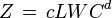
with Z is in [mm6 m-3] (e.g. Atlas 1954, Sauvageot and Omar 1986). This relation is, however, extremely dependent on the DSD. For example, if an air volume of 1 m3 contains 0.1 g of liquid water and only droplets 5 µm in radius, the reflectivity will be 8 times smaller than if the volume consists only of droplets 10 µm in radius. The coefficients c and d may be derived empirically from in-situ aircraft measurements by measuring the DSD, calculating LWC and Z (assumption Rayleigh scattering) and finally using a least squares to determine a and b. Instead of aircraft measurements other attempts have been made using microphysical cloud models, which resolve the drop size spectrum (Liao and Sassen 1994) and thus allow the calculation of Z and LWC. Fox and Illingworth (1997a) show scatter plots of LWC and Z calculated from DSD-aircraft measurements, which show maximum uncertainties of up to one order of magnitude in LWC for a single measurement if only droplets smaller than ~50 µm in radius are considered. They claim relative LWC accuracies of ~50 % for typical marine stratocumulus.
Since LWC is proportional to D3 and Z to D6, the occurrence of just a few larger precipitating (drizzle) drops, which do not contribute significantly to LWC, will dominate the radar signal. Many low level stratocumulus clouds contain drizzle drops and consequently Z - LWC relations must be adapted accordingly during precipitation.
Most modern cloud radars have Doppler capabilities and thus the possibility of measuring the Doppler velocity spectrum. Here, the possibility is given to detect precipitating particles by relating the Doppler velocities of particles to their fall speed, which is determined by particle size.
As shown by Hogan et al. (2005), another approach towards retrieving LWC from radar measurements is to use two radars at different wavelengths. Since attenuation is proportional to LWC within the Rayleigh backscattering regime, the differences between the Z measurements at a certain height give information on attenuation and thus on LWC.
Infrared spectrometer: Next to being sensitive to temperature and traces gases (i.e. water vapor, carbon dioxide, methane, nitrus oxide) highly resolved spectral infrared measurements as provided by an AERI are also sensitive to liquid and ice clouds. Thus, together with reasonable a priori assumptions for temperature and humidity, an AERI is able retrieve the cloud properties cloud effective radius (Reff) and cloud optical depth (COD). An AERI spectrum is sensitive to the liquid cloud properties Reff and COD, whereas MWR observations of liquid clouds are generally sensitive to the integrated liquid water path (LWP). However, within the optical limit, COD=3LWP/2(rholReff) directly relates MWR and AERI observations, with rhol the bullk density of liquid water. At approximately LWP=60gm-2, the signal of the infrared spectrometer is fully satured. This implies, as mentioned by Turner et al., that an AERI can only be used to retrieve the microphyical properties of thin liquid water clouds, which can however, effectively regulate the solar radiation balance.
Shortwave irradiance: Cloud optical depth can also be derived by using shortwave irradiance measurements. Together with LWP from an MWR, additionally the mean effective radius can then be derived. Several studies have been carried out to estimate cloud optical depth (COD) by broadband (Leontyeva and Stamnes 1994, Dong et al. 1997, Boers 1997, Barker et al. 1998, Qiu 2006) and narrow band (Min and Harrison 1996, Marshak et al. 2000, Daniel et al. 2002, Marshak et al. 2004, Min et al. 2004, Chiu et al. 2010, Matamoros et al. 2011) global (i.e. direct+diffuse), diffuse or direct measurements of irradiance in the shortwave (SW) region. Here we focus on methodologies using broadband SW irradiance, because of the large availability of such type of measurements. The empirical and semi-empirical methodologies presented by Barnard and Long (2004) and Barnard et al. (2008) permit to estimate the COD using the ground-based diffuse and global SW irradiance, respectively, without the need of using other type of measurements or radiative transfer model simulation. Other advantage of these techniques concern the methodology itself, which reduces the impact of the pyranometer calibration. These characteristics make such methodologies attractive for use in routine calculations over one or more sites and for collection of long time series of data. Major drawbacks of this approach are the assumption of a plane-parallel and homogeneous cloud, possibly satisfied in cases of fully overcast conditions, and the lack of information related to the vertical distributions of the clouds. Moreover, the applicability of these algorithms is limited to surface types characterized by albedo lower than 0.30, to solar zenith angles below 75° and to COD values larger than about 5. For further detailed see Barnard and Long (2004) and Barnard et al. (2008). The cloud effective radius can be estimated using COD and LWP values. Assuming a constant LWC(z) within the cloud and a value of the extinction efficiency factor of 2 in the SW region, the effective radius is Reff=3/2*(LWP/COD). Actually the vertical profile of the effective radius varies within the cloud, generally increasing from the cloud base up to the proximity of the cloud top. Under the assumption of a linear increase in LWC(z), i.e. adiabatic profile, it is possible to derive the maximum value of Re(z) as Re(z,top) = 9/5*(LWP/COD)
3.7.3 Synergetic profiling retrieval algorithms
Within the scope of the EG-CLIMET four different retrieval methods for profiling LWC, Reff and N all based on active and passive ground-based microwave remote sensing measurements have been thouroughly assessed. The combination of passive MWR and active cloud radar together with a backscatter lidar are currently the most robust way to profile liquid cloud microphysical properties, concerning both 24/7 instrument performance and well as algorithm applicability. All methods use the same information on cloud phase & type, cloud boundaries, radar reflectivity, ceilometer-backscatter and MWR-derived LWP, respectively MWR brightness temperature. This information is derived by the Cloudnet categorization product. Additionally these measurements are available at all atmospheric profiling observatories.
In order to have a "truth" to validate against, all retrieval methods have been applied in a synthetic model environment. Measurement simulations of the ground-based remote sensing instruments using microphysical variables from cloud resolving model output provided this reference. The simulations were carried out within the framework of ECSIM (EarthCare Simulator). After applying the microphysical retrievals to the measurement simulations, an independent evaluation of performance was carried out in order to identify strengths and weaknesses and to improve the retrieval algorithm quality in general. Additionally, the methods are applied to real measurements and evaluated through a short-wave radiative closure using simultaneous broad-band pyranometer measurements.

Cloudnet - scaled adiabatic
The Cloudnet algorithm is the standard method within the Cloudnet products to retrieve LWC. In case a non-precipitating liquid cloud is detected by the Cloudnet categorization scheme, cloud base, cloud top and cloud temperature (extracted from atmospheric model output) are used to calculate the adiabatic liquid water content as a function of height above cloud base. Since this LWC represents a theoretical upper limit to cloud LWC, the LWC profile is linearly scaled to meet the the LWP determined independently by a MWR.
TUD-RSCPP algorithm The retrieval method relies on a combination of the cloud radar reflectivity, the microwave radiometer estimated liquid water path and on the cloud geometrical thickness from lidar and cloud radar. These observations are used as input data for different vertical cloud models to retrieve profiles of the LWC, the droplet concentration, the effective radius, the optical extinction and the optical depth. The three cloud models are characterized by their predefined in-cloud vertical structure of the assumed gamma DSD parameters (concentration, shape parameter and mean radius). This assumption is necessary to reduce the number of unknowns since the vertical information of the DSD properties from surface remote sensing observations are still lacking. The common assumptions in all three cloud models on the vertical distribution of the DSD parameters are that the cloud droplet concentration and DSD shape parameter remain constant within the cloud layer. The differences in the in-cloud vertical structure of the cloud models are related to the cloud layer mean droplet radius. In the vertical uniform (VU) cloud model, the cloud layer mean droplet radius is uniformly distributed over the cloud layer thickness while the scaled-adiabatic stratified (SAS) and homogeneous mixed (HM) cloud models parametrize the vertical profiles of the mean droplet radius in consideration of possible impacts of the cloud dilution. The SAS cloud model accounts for the entire range of mixing processes available in the atmosphere by a constant reduction in the particle size with height. In case of the HM cloud model, the impact of mixing is associated with the observed vertical variation in the radar reflectivity profile, which is attributed to changes in the mean particle size. The main assumptions constrain the application of the algorithms to liquid water clouds without drizzle formation and it is expected that drizzle-sized particles will produce biased results, because they are dominating the cloud radar reflectivity while their contribution to the LWC, the droplet concentration and the effective particle size are rather small.
IPT - Integrated Profiling Technique: The IPT (Löhnert et al., 2004, Löhnert et al. 2008) is a variational scheme for retrieving profiles of temperature, humidity and cloud microphysical properties. The core version of this technique includes the physically consistent combination of microwave radiometer, cloud radar and lidar/ ceilometer together with information on the background state (a priori information). It is a variational technique that, similarly to data assimilation techniques, requires uncertainty estimates of the measurements, forward model and background state, which need to be carefully specified. If assuming a Gaussian distribution of atmospheric variables, measurements and their corresponding error, the solution will bring forth not only the most probable solution, but also the error covariance matrix for each derived variable. The retrievable parameters include profiles of temperature, humidity and LWC, as well as Reff. By adapting an empirical relation between Z and LWC for cloud, respectively precipitation, it can retrieve LWC also in drizzling cases.
SYRSOC - Synergistic Remote Sensing of Cloud:
SYRSOC (SYnergistic Remote Sensing Of Cloud) is a multi-module technique developed at the National University of Ireland Galway and retrieving the three primary microphysical parameters from liquid clouds (Martucci and O’Dowd, 2011, Martucci et al., 2012, Ovadnevaite et al., 2011), i.e. the cloud droplet number concentration (CDNC), the effective radius ( ) and the cloud liquid water content (LWC). In addition to the three main microphysical variables, SYRSOC provides a number of parameters describing the cloud droplet spectral properties (relative dispersion), the degree cloud of subadiabaticity, the Doppler spectrum of droplets, the cloud optical depth and the cloud albedo. Extinction from standard 355-1500 nm inverted backscatter LIDAR signal or directly from Raman signal is used as input data for SYRSOC. Other input data are the temperature and humidity profiles from co-located operational microwave-radiometer and the reflectivity/signal-to-noise-ratio and depolarization ratio from co-located Ka-band Doppler cloud RADAR. Data from the 1064-nm and 15-km vertical range Jenoptik CHM15K LIDAR ceilometer, the RPG-HATPRO water vapour and oxygen multi-channel microwave profiler and the MIRA36, 35 GHz Ka-band Doppler cloud RADAR are currently used at the GAW Atmospheric Station of Mace Head (Ireland) to supply the necessary input to SYRSOC.
3.7.4 Technical implementation and performance
In the following, the main results of the retrieval algorithm application to the simulated data sets are discussed with respect to the different microphysical parameters.
LWC

A comparison between the standard Cloudnet scheme and the RSCCP method acording to Brandau (HM cloud model) shows an improvement in LWC retrieval skill using the latter method (Fig. 3.7.3). In contrast to Cloudnet, which relies on a linearly scaled adiabatic assumption, the Brandau method uses radar reflectivity profiles from a cloud radar assuming a relationship between the 2nd and 3rd moment of the DSD based on aircraft measurement (Brenguier et al. 2011). This assumption holds only in non-precipitating clouds. Note, three of the four assessed methods require the LWP derived by independent measurements of an MWR. In non-precipitating cases, the accuracy of LWP is the most crucial factor for retrieving both LWC and Reff. In case the LWP is accurately know, random and systematic error can both be on the order of ~10% for the Brandau method. The IPT method was shown to be very sensitive to the a priori assumption, is however, independent of LWP, whereas the SYRSOC method is very sensitive towards an accurate retrieval of lidar extinction from lidar backscatter. All retrieval methods were shown to be very sensitive towards a correct description of cloud base and cloud top and the corresponding distinction between cloud droplets and precipitation.
Reff & N

For non-precipitating cases, the Brandau retrieval method delivers the most satisfactory results for Reff (Fig. 3.7.4, left). Within the cloud boundaries, Reff can be derived with overall accuracies of ~15%. The Brandau method as well as the IPT assumes constant values of N throughout the cloud. Although this is actually the case within the clouds analysed (Fig 3.7.4, right), systematic errors of more than 50% occur. Improvements are only possible if a more situation-specific relation between the 2nd and 3rd moment of the droplet size distribution is used instead of the one proposed by Brenguier et al. 2011.
Precipitation Frequently, liquid clouds contain precipitation size drops (drizzle). In these cases the assumptions on the relations between 2nd and 3rd moment of the droplet size distribution is no longer valid, leading to large overestimation (underestimation) of Reff (N) because a small number of larger droplets dominate the radar reflectivity factor signal. However, both IPT and Brandau method still deliver fairly robust results in LWC with overall errors in the range of 20-50%.
3.7.5 Summary and Outlook

Due to their capability to provide continuous observations, ground-based remote sensing observations of clouds are widely used and well suited for:
- Long-term observations (Validation of new methods, climate applications), e.g. Fig. 3.7.5 gives an impression about the amount of liquid water at Lindenberg during one year. It shows a histogram of non-rejected retrievals indicating that no liquid water was observed at about 24% of the cases. For only for 8% the LWP was greater than 200 gm-2.

- NWP model validation. For validation studies LWC, N and Reff measurements are needed as component of a variety of continuously observed parameters. Investigations, which aim at revealing possible deficiencies in the model parameterization, rely on the long-term availability of corresponding parameters. The periods may cover time intervals ranging from months up to several years. LWP from MWR can be provided for such long periods of time. In the frame of a validation study (Vogel et al., 2011) of operational weather forecast models (COSMO-EU) a systematic prediction error of the 2 m temperature during winter months was found. The overestimation of the noon temperature results from an error of the radiation balance at surface of about 20-40 W m-2. In order to find reasons for the overestimation the radiation balance was split into solar and thermal components. In fact, model radiation peaks appear in low stratiform clouds because their cloud water content is considerably to low compared to the MWR-derived LWP. Furthermore, if the model produces a realistic LWP then the radiance balance simulated by the model agrees with the observation (Figure 3.7.6).
Next steps Currently, research focus is on developing retrieval methods that allow determining microphysical properties of the non-precipitating and precipitating parts of the liquid cloud. This can only be achieved by using additional information from the full Doppler spectrum of the cloud radar. Furthermore, physically consistent a priori data (i.e. long-term statistics) of cloud profiles is needed from in-situ measurement to be able to better constrain the retrieval methods. These methods should be ideally developed within a variational framework, which is flexible concerning the used measurements and retrieval assumption and additionally allowing an inherent error approximation.
4 Networks
4.1 Operational networks
4.1.1 The European network of wind profilers CWINDE

The EUMETNETE-WINPROF programme is providing vertical profiles of wind measurements from wind profilers and weather radars from a network of stations across Europe. Its main goal is to improve the overall usability of wind profiler data for operational meteorology and to provide support and expertise to both profiler operators and end users. Since 2002, this programme is operating the network CWINDE (fig. 4.1.1) which displays time series of realtime quality controlled wind profiles from more than 25 sites in Europe.
Monthly statistics on availability and data quality are sent to the data owners. A list of wind profilers and weather radars whose winds are operationally assimilated into the main Numerical and Weather Prediction (NWP) models in Europe is also updated on a regular basis.
4.1.2 The Swiss nuclear powerplant meteorological surveillance tool CN-MET

The main purpose of CN-MET (Centrale Nucléaire et METéorologie) is to bring up to date the system delivering weather information necessary to the population safety in case of a nuclear hazard. CN-MET represents the coupling of a specifically adapted measurement network (mainly ground-based remote sensing) and a predictive tool in the form of a fine grid numerical weather prediction model currently operated at MeteoSwiss (COSMO-2). This new tool, calling upon modern measurement and modeling techniques of the atmosphere, represents a solution which will keep all its relevance for the next decades.
In case of a nuclear accident, the necessary atmospheric data used to calculate the diffusion of a contaminated air mass will be provided by a fine grid numerical model, covering the whole Swiss territory. The measurement network within CN-MET combines in-situ measurements and ground-nased remote sensing systems (wind profilers and microwave radiometers). It is directly adapted to provide the best information (initial and boundary conditions, as well as test measurements) for this model. CN-MET not only ensures the emergency preparedness for the concerned population on a local scale, but also enhances it on a regional scale corresponding to the Swiss Plateau.
For more information: Calpini et al, 2011.
4.2 Candidate networks
4.2.1 Ceilometer network
The number of automatic Lidars and ceilometers with profiling capability installed over Europe has increased over the past two years. National Meteorological and Hydrological Services (NMHS) in Germany, France, the Netherlands and the United Kingdom, in particular, are deploying Lidars and ceilometers to cover their national territories with the objective to reach a spatial density of nearly one device every 100 km (e.g. Haij and Klein Baltink 2007; Flentje et al. 2010). Figure 4.2.1 (from Haeffelin et al., 2012) provides a convincing representation of the density of automatic backscatter lidars and ceilometers. These investments have been made because of the Lidars/ceilometers ability to detect volcanic ash, but the network is potentially of great value in monitoring clouds and pollution and evaluating their representation in NWP models. Ultimately, incorporation of such data could lead to improved prediction of air quality and hazardous weather.
Although the name ceilometer suggests that their sole purpose is to detect cloud-base, modern ceilometers are able to provide continuous accurate and reliable profiles of backscatter from aerosols and clouds. In the past, Lidars were strictly research instruments. Similarly modern Lidars are becoming more automated and can now contribute efficiently to continuous monitoring of air quality and weather.
Several communities have expressed interest in exploiting data that can be derived from automatic Lidars/ceilometers in Europe: for evaluation of the representation of clouds and aerosols in operational weather forecast models run by National Met Services, for evaluation of climate models, for aerosol transport surveillance and air traffic safety (eg VAAC services, national aviation control entities), for air quality applications (eg EU FP7/GMES MACC-II programme), for greenhouse gas monitoring applications (eg. GAW, ICOS programme). Hence, efforts should be made to provide Lidar/ceilometer data in a harmonized way in Europe.
Automatic Lidar and Ceilometer map over Europe
About 50 institutions, mainly the European NMHSs and aviation control entities, were contacted for their national Lidar and ceilometer networks and a station map was generated using the google earth visualization tool (see Figure 4.2.1). Several WMO member states of the RA VI did not respond to the survey (Albania, Georgia, Lithuania, Luxembourg, Russia, Serbia, Hungaria, Ukrainia, Italy, Bulgaria), thus were not providing any information about local capacities. Enhancements of national ceilometer networks are currently planned in Belgium, Finland, France, Iceland, and Italy. Google Earth was chosen for visualizing the ceilometer positions and the instrument types. The map contains more than 1000 positions (as of March 2012) of ceilometers and lidars in Europe (EARLINET, CIS-Linet, Pollynet, Leonet) but also America (MPLnet) and Asia (AD-net lidars), thus showing the potentially available global vertical profiling capacities. There is however no storage of raw data for roughly half of all instruments gathered, making it impossible to retrieve information about aerosol layers at these positions. These stations are generally marked by using different white symbols representing the different instrument types in the animation. Several EARLINET stations, the entire AD-net and all active MPLnet stations provide quick looks of the backscatter signal. Furthermore, all Jenoptik ceilometers in Germany and some LD40 instruments in the Netherlands operated by KNMI provide links to quick look images (range-corrected backscatter intensities) in near-real-time. Links to quick looks of the UK Met. Office (UKMO) instruments will be added at a later stage. In case of emergency (e.g. volcanic ash plumes) the map may provide information about the spatial distribution of ash clouds and the height regime of such clouds. The map can easily be enhanced by users by adding more stations and/or additional information (e.g., station meta data). The Lidar/ceilometer map is electronically available (as google earth kml-formatted file) on request from the author but requires currently at run time a google earth installation at the user’s site. It is planned offering download of the latest stable version through a dedicated web page.

| Table 4.2.1: Legend for Lidar and Ceilometer map | |||
|---|---|---|---|
| blue symbol "square": | Vaisala CT12K | blue symbol "blank": | Vaisala CT25K |
| blue symbol "star": | Vaisala CL31 | blue symbol "diamond": | Vaisala CL51 |
| blue symbol "circle": | Vaisala CT75K | cyan/white symbol "square": | Vaisala LD12 |
| cyan symbol "blank": | Vaisala AW11 | cyan symbol "circle": | Vaisala LD40 |
| white shaded circle: | Vaisala CTC21 | green symbol "blank": | Eliasson CBME80 |
| green needle: | Jenoptik CHM15K | yellow needle: | Jenoptik CHM15KX |
| yellow symbol "star": | other Lidar | red symbol "A": | AD-net |
| red symbol "C": | CIS-Linet | red symbol "E": | Earlinet |
| red symbol "L": | Leonet | red symbol "M": | MPLnet |
| red symbol "N": | NDACC | red symbol "P": | Pollynet |
| black/white squares: | Telvent Cirrus 100 | black/white circles: | MTECH 8200 |
| white: | backscatter data stored, instrument types as given above | ||
| white donut: | unknown instrument type | ||
The data was transfered to an openlayers-based solution, which is free of charge, and the result is now visible and accessible under DWD - Ceilometer-Viewer
Progress and Challenges
Towards a European network of automatic lidars and ceilometers: Harmonizing recording formats and data sharing protocols, data quality management, calibration, target classification and parameter retrievals for clouds and aerosols.
There is an increasing interest in Europe for automatic Lidar/ceilometer data for NWP evaluation and assimilation and for atmospheric surveillance (eg. aerosol transport). Most European countries are planning or are in the process of deploying reasonably dense networks of profiling ceilometers or automatic lidars.
This topic is at the cross road between “operational observation specialists” (Met Services) and “Lidar data interpretation experts” (Research programs).
Several communities have expressed their interest in exploiting data that can be derived from automatic Lidars/ceilometers in Europe: for evaluation of the representation of clouds and aerosols in operational weather forecast models run by National Met Services, for evaluation of climate models, for aerosol transport surveillance and air traffic safety (eg VAAC services, national aviation control entities), for air quality applications (eg EU FP7/GMES MACC-II programme), for greenhouse gas monitoring applications (eg. GAW, ICOS programme). Hence, efforts should be made to provide Lidar/ceilometer data in a harmonized way in Europe.
EG-CLIMET has brought together Met Service representatives involved in Lidar and ceilometer activities and Lidar data analysis experts involved in the EU FP7 ACTRIS programme.
Main conclusions: The participants are highly motivated by the importance of establishing a European network of automatic lidars and ceilometers that would enable data sharing and harmonized processing. A website will be developed to give visibility to the network, present the state of the network and give access to visualization of the measurements, initially at just a few sites (e.g. DWD - Ceilometer-Viewer).
The group proposes that data sharing, calibration and processing shall be handled in a framework similar to the WINPROF system of EUMETNET. This system would include data sharing based on BUFR format, and, harmonized processing using common algorithms (possibly also centralized processing).
Formats: The group will propose a common BUFR format for operational purposes allowing efficient data sharing.
The group will propose a common NetCDF format for scientific applications that will contain all data and metadata.
Calibration and processing: Calibration of automatic lidar/ceilometer measurements is important to enable scientific exploitation of the data. The group will develop common procedures to produce calibrated backscatter profiles.
Processing of calibrated lidar/ceilometer data to produce (1) target classification, liquid cloud, ice clouds, aerosol; (2) aerosol and cloud backscatter profiles; (3) aerosol and cloud extinction profiles; (4) aerosol speciation is of high importance, in order to inform users about observed aerosol properties. The group will propose common procedures to retrieve these properties (inspired by the experience of the FP6 programmes, EARLINET and CLOUDNET).
The way forward: Following EG-CLIMET presentations to EUCOS, the body responsible for the European observing system, E-PROFILE has been launched which will run from 2013-2017 with a kick-off meeting in April-May 2013. E-PROFILE will be responsible for Wind Profiler data quality and for coordinating real time exchange of backscatter profiles from lidars and ceilometers. E-PROFILE will be involved in the logistics, a proposed COST action ‘TOPROF’ would be concerned with operational problems of data quality, calibration and the formats for data exchange.
4.2.2 MWRnet
MWR can provide timely and enough accurate atmospheric temperature and humidity data, especially good in the planetary boundary layer (PBL), which remains the single most important under-sampled part of the atmosphere, outside the reach of surface sensors and with poor satellite coverage. At the EG-CLIMET MC Meeting in Oslo (March 2009), some MC/WG members concurred on that the use of ground-based MWR in NWP and climate studies was hampered by unsufficient communication between users, manufacturers, and experts, lack of coordination for networking, unknown number of operational MWR. Thus, a long-time overdue cooperation and coordination effort started under the auspices of EG-CLIMET: MWRnet, an International network of MicroWave Radiometers. MWRnet aims to address the lack of coordination between the MWR operations and increase the utilization of quality controlled MWR data. The long-term mission of MWRnet is the set up of an operational network sharing good practices (in terms of procedures, formats, quality control, protocols, software, etc...) and life cycle of MWR data, facilitating the access of well documented and quality controlled MWR observations and retrievals (with errors).
MWRnet currently links about 61 members, operating more than 94 MWR world wide (including dual-channel units, water vapor profilers, single-channel temperature profilers, multi-channel temperature profilers, and temperature and water vapor profilers), of which about 30 in Europe (temperature and water vapor profilers, for the most). More information on MWRnet and the network map are available at: MWRnet website
MWRnet started within EG-CLIMET and most of the activities were carried out within this COST action. In particular, 3 SWG meetings and 3 STSM were performed:
- SWG 00: From raw data to meteorological products
- SWG 02: MWR data processing
- SWG 17: Towards operational use of MWR data
- STSM 06: Assessment of Microwave Radiometer Temperature Profiling
- STSM 11: Estimate of PBL Mixing Height from MWR data
- STSM 13: Development of a ground-based Radiative Transfer Model (RTM) for NWP
The major achievements of MWRnet within EG-CLIMET were:
- Development of calibration control methods
- Advances in retrieval algorithm development
- MWR Data Assimilation experiment
- Assessment of O-B statistics
- Initial efforts towards a ground-based MWR Forward Model suited for NWP
- EU FP7 proposal EMERGE (unfunded)
In particular, the proposal EMERGE (European MicrowavE Radiometer network within GEo) grouped eight members (CETEMPS-Univ. of L’Aquila (IT), Univ. of Köln (D), KNMI (NL), IMAA (IT), FMI (FI), DWD (D), Meteoswiss (CH), MetOffice (UK)), five of which from National Weather Services. EMERGE passed all quality criteria but unfortunately did not reach the funding level.
MWRnet pursued building connections with NWP data assimilation (DA), climate, and radiopropagation communities:
- NWP DA:
- Contribution to the US Tropospheric Profiling Technology Workshop (organized by the US NSF and NWS)
- Invitation to chair a session on the German DA Workshop
- DA experiment in collaboration with Meteo France (HyMeX)
- Mention in the EUCOS roadmap for 2013-2017 as an interesting network for EUCOS expansion
- CLIMATE:
- Invitation to join the GRUAN (GCOS Reference Upper Air Network) Task Team 5 focusing on ancillary measurement (w.r.t. radiosondes)
- Contribution to the MWR handbook for GRUAN
- RADIO PROPAGATION
- Contribution to the final report of COST Action IC0802 – “Propagation tools and data for integrated Telecommunication, Navigation and Earth Observation systems” with a MWR handbook focusing on MWR estimates of atmospheric attenuation
At its present stage, MWRnet faces both technical and bureaucratic challenges:
- Implement common data life-cycle (data format, quality control, retrieval)
- Establish a trusted ground-based MWR Forward Model suited for NWP
- Data sharing policy
As the outcome of the MWRnet meetings, the following recommendations were collected for good practices with MWR operations.
| Table 4.2.2: MWRnet recommendations for MWR operations | ||||
|---|---|---|---|---|
| # | Type | Recommendation | Note | |
| MM1 | Measurement mode | Perform zenith viewing alternating with elevation scans regularly, possibly as frequent as 5 min. Store observations at all channels. If possible, perform 2-side scans. | ||
| MM2 | Measurement mode | Perform frequent observations of the calibration load (5min intervals). Use integration time ~10 sec (as calibrations need to have longer integration times than the observations for a safe reduction of rms noise). | ||
| MM3 | Measurement mode | Ideally, all raw voltages of receivers and temperatures in the radiometer system should be recorded continuously in order to make a post-calibration possible. | ||
| MM4 | Measurement mode | Level 0 data should always be stored. Always store data even if quality flags are on. Avoid discarding data. | ||
| CC1 | Calibration control | Carefully follow instructions for cryogenic calibration. If possible check Tb after cryogenic calibration against a reference (e.g. clear sky radiosonde simulations). | ||
| CC2 | Calibration control | Before each cryogenic calibration: observe the cold load for ~2min to characterize the instrument drifts since the last calibration. Note that this need a dedicated featured software since the observed TB will NOT be the LN2 temperature. In fact, the interface reflection on the LN2-surface, residual mirror emission, overspill-termination and other correction factors need to be applied. | ||
| CC3 | Calibration control | Be careful when using calibration coefficients obtained by a single sky dip (tipping curve). Make sure the threshold for a horizontally homogeneous sky are set very tight, Averaged time series of sky dip calibration coefficients may be used to avoid jumps in the data. Perform full sky-scans to assess the validity of the “homogeneous sky” assumption. | ||
| CC4 | Calibration control | Inspection by manufacturer every 1.5-2 years is recommended. | ||
| CC5 | Calibration control | Re-processing of MWR observations and retrievals may be possible if a comparable set of collocated radiosonde profiles is available. Alternatively model analyses could be used. | ||
| CC6 | Calibration control | Climate application should rely on careful calibration monitoring (including radiative transfer comparison and close maintenance). | ||
| CC7 | Calibration control | Gain calibration should be performed once every 3-5 minutes for some 5-10 sec integration time. | ||
| QC1 | Quality control | Use sanity checks to monitor the reliability of the instrument hardware and thus of observed Tb. Use flags provided by manufacturers as well as developed by users. | ||
| QC2 | Quality control | Use quality control checks to estimate the value of retrievals in opaque (rainy) situations. Use flags provided by manufacturers as well as developed by users. | ||
| QC3 | Quality control | Rain flag is necessary, especially for humidity, but is may overkill acceptable retrievals. Check the quality of retrievals during rain flagged periods. | ||
| RA1 | Retrieval algorithm | Uniform multi-linear regression (or NN) retrievals based on radiative transfer calculations should be implemented. These are robust to handle and their accuracy is mostly optimized. Alternatively, direct regression retrievals based on the relation between measurements and model output should be considered. | ||
| RA2 | Retrieval algorithm | Ideally, a variational approach should be adopted for all the MWR. However, future testing is required – specifically concerning the handling of liquid clouds | ||
| RA3 | Retrieval algorithm | The estimate of the retrieval error should be provided. | ||
| RA4 | Retrieval algorithm | The estimate of in-depth retrieval characteristics should be provided (averaging kernels, degrees of freedom) | ||
| RA5 | Retrieval algorithm | Avoid RH profiles computed from T and WV retrieved profiles. | ||
| DF1 | Data format | Produce data in a easy-to-share format with metadata. | ||
| DF2 | Data format | netCDF format complying to the Climate-Forecast (CF) convention is preferable. | ||
| DF3 | Data format | Common data and metadata format should be decided building on the experience of ARM, LUAMI, COPS. | ||
| DF4 | Data format | Data should be processed and stored in a reliable and centralized server. | ||
5 NWP Applications
5.1 Quantifying the impact of wind profiler observations
5.1.1 Wind Profiler Impact seen by FSO preliminary results
Until recently there had only been a few studies of the impact of wind profiler observations in NWP and these studies concluded that the impact is very small, or even neutral in the UK Met Office global unified model (UM). “Significant impact cannot be detected from the European wind profiler network” Technical Report No. 532 2009, Richard Dumelow. In this denial experiment, wind profilers were removed as a whole observing system along with VAD wind from weather radars.
Within the last couples of years several Met services like NRL, ECMWF, the UK Met Office have developed forecast sensitivity to observation (FSO) tools which estimate the reduction of forecast error associated with individual observations. At the Met office, this tool has been recently developed for the global model by Andrew Lorenc and Richard Marriott and is run to correspond with parallel suites containing significant changes to the UM and /or data assimilation. It allows comparison of the impact of different observing systems (Lorenc and Marriott 2012) for different versions of the model. For the first time, the impact of each wind profiler can easily be examined.
In this section we show the impact, measured by FSO, of wind profilers on 24-hour global forecasts over a period of one month and compare it with radiosonde impact. The theoretical foundation for the Met Office FSO tool is fully described in Lorenc and Marriott 2012.
5.1.2 Wind profiler impact on 24-hour global model forecasts

Using the chain rule of derivatives (adjoint techniques), values of forecast error sensitivity to observations (usually at a forecast length of 24h) can be computed for each assimilated observation simultaneously. The values represent the change in forecast error for a unit observation innovation. Multiplying the sensitivity by the observation innovation gives an estimate of the forecast error difference due to the observation. This is an estimate of the observation’s impact in the full system, i.e. assimilation + forecast model. The innovation is the difference between the equivalent model observation computed from the forecast valid at the analysis time issued from the previous analysis and the observation use in the current analysis cycle. The forecast error is computed using an energy norm which includes elastic and potential energy, thermal energy, the latent thermal energy of condensation and kinetic energy (Lorenc and Marriott 2012). The forecast error can be computed on any domain. In this study the domain is the full globe for model levels up to 150 hPa.
This tool has been developed for the operational global model which uses a 4D-Var assimilation scheme (Rawlins et al 2007). The FSO tool was run over a period of approximately one month from the 22/08/2010 until the 29/09/2010 using a reduced-resolution version of the UM that was operational at the Met Office between 16 March and 20 July 2011. The full forecast model was run at N512 resolution (approx. 25km in the horizontal and the adjoint model at N216 (approx. 60km in the horizontal. The 4D-Var assimilation scheme uses a 6 hour window and was run at N216 resolution in both the forward and adjoint runs. The wind profilers which are suitable for data assimilation are quality controlled using a background check (if the innovation is too large the observation is rejected). The wind profiler data are hourly thinned.

Figure 5.1.1 shows FSO-estimated values of the difference in 24h forecast error associated with the use of wind profiler observations within areas of 2.5 by 2.5 degrees. If in that area two profilers are present, their impacts are combined. N.B. the field shows estimated values of forecast error impact attributed to observations in those locations, not the change in forecast error itself. The error difference measured by the FSO tool was accumulated over the full period for each of the wind profilers and weather radars assimilated in the UK Met Office global model. The impact is quite variable but most of the wind profilers have a beneficial impact (negative value corresponding to a reduction in forecast error). The strongest beneficial impact comes from the Japanese network whilst a few wind profilers have a detrimental impact. The profiler in the middle of Alaska is clearly giving a detrimental impact. A few wind profilers in the US are also measured as having a detrimental impact. In Europe, impacts are mostly neutral/beneficial except for over Switzerland.
The detrimental impact of the wind profiler located in Alaska is due to the quality of the data. Figure 5.1.2 shows one example of these observations. A fair amount of the winds are blowing in spurious directions. Most of them are flagged by the data assimilation quality control but some suspect winds are assimilated. The comparison of the wind against the first guess (Figure 5.1.3) reveals strong bias and a large root mean square deviation. This wind profiler is now blacklisted by the Met Office and is in need of maintenance. (It stopped sending data in 2012.) Some of the other wind profilers from the NOAA network are also giving slightly detrimental impacts; the origin of these detrimental impacts has not yet been studied. The wind profiler in Switzerland at Payerne is located in the vicinity of very complex terrain not well represented by the global model and it is not surprising that such detailed information might have a detrimental effect on the global model. The comparison with the global model in Figure 5.1.4 clearly shows large biases in the boundary layer.


Figure 5.1.5 shows total 24-hour forecast impacts for all European wind profilers. The largest beneficial impact is for wind profiler 03020 South Uist high mode UK (North West Scotland), followed by 10266 Ziegendorf (North Germany). A couple of wind profilers are giving detrimental impacts where they are situated in regions of complex orography (Switzerland 6610, 6632 ). The detrimental impact for the three other wind profilers 11036, 12842, 12982 haven’t yet been investigated.

In the UK, total wind profiler impact for the period is larger than that for radiosondes; (see Figure 5.1.6 and 5.1.7) by a factor ~3 when comparing the South Uist wind profiler and Lerwick radiosonde, which are both located in Scotland, and for Camborne (Cornwall).


At Lindenberg in Germany, the mean wind profiler impact per sounding is as large as the mean impact per radiosonde profile (Figures 5.1.8 and 5.1.9) even though radiosonde observations include temperature and humidity readings as well as winds. (Part of the reason for this could be that the Lindenberg wind profiler is located at a manned observatory (GRUAN station) and is very well maintained.) When accumulated over the full period, the wind profiler impact is larger than the radiosonde impact by a factor ~7 (Figures 5.1.10 and 5.1.11) due to the higher frequency at which wind profiler soundings are performed. The variance of the Lindenberg radiosonde impacts is large meaning that there may be error in our estimation of this mean impact. This result should therefore be confirmed over a larger period of time. Also, it is possible that errors in the impacts of individual observations might be correlated (in height and in time). The total impact, which is just the sum of all the individual impacts, might then be exaggerated. This needs more investigation. However, as the Lindenberg wind profiler and radiosonde are collocated, their impact estimates should each suffer from similar error-correlations. Comparison of their impacts is therefore justified.
When comparing the impact of Lindenberg with Ziegendorf or South Uist, the impact is relatively small. This is not surprising as, at Lindenberg, the atmosphere is already well described in the model due to assimilation of the radiosonde four times a day. The same applies for Camborne where both wind profiler and radiosonde are assimilated. There is a tendency to measure larger impacts for wind profilers and radiosondes located close to the sea, e.g. Lerwick, South Uist, Eimden, Ziegendorf.
5.1.3 Conclusion
The FSO tool allows efficient estimation of the impact of each wind profiler. Some wind profilers have a detrimental impact because of quality issues (as in Alaska) or representativeness problems (as at Payerne) but most are measured as having a beneficial impact. The largest impacts come from the Japanese network which are very homogeneous in quality. In general the impact is larger near the coast and in other less well-observed areas. For the studied period, wind profilers of good quality were found to have as much impact per profile as radiosondes with the total wind profiler impact being much larger when accumulated over time. Correlation of errors may cause the beneficial or detrimental impact of observations to be exaggerated. However, these preliminary results tend to indicate that wind profilers could be giving large impacts where they are well maintained and placed in strategic locations. An extended period should be studied to confirm these findings.
5.2 Operational assimilation of wind profiler observations

Wind profiler observations are operationally assimilated at the European level since a few years (see CWINDE). At the regional scale, an operational system combining wind profiler measurements and a 2km-resolution NWP model was designed in Switzerland (see Figure 5.2.1). Its main purpose is to deliver weather information necessary to the population safety in case of a nuclear hazard. It represents the coupling of a specifically adapted measurement network (mainly ground-based remote sensing) and a predictive tool in the form of a fine grid numerical weather prediction model currently operated at MeteoSwiss (COSMO-2). During the project phase, the positive impact of the three wind profilers on the quality of the forecast over the Swiss Plateau was demonstrated. This system is operational since 2009 Calpini et al, 2011..
5.3 MWR data assimilation test
A first trial of assimilating microwave radiometers (MWR) measurements into numerical weather prediction was carried out in preparation to the Hydrological cycle in Mediterranean EXperiment (HyMeX) Special Observing Period 1, held in September-November 2012 in the Western Mediterranean (WMed) arget area.

The NWP system used for this study is Arome-WMed, a particular version of the Arome system covering the western part of the Mediterranean Sea (see fig. 5.3.1). Arome-WMed has a horizontal resolution of 2.5 km, a non-hydrostatic dynamical core, detailed physics inherited from the research Meso-NH model, and is coupled with the global Arpege NWP system. It has a three-dimensional variational (3DVar) data assimilation system [10] with background covariances specially computed for the WMed domain. 3DVar analyses are performed every three hours and provide new initial states for subsequent forecasts. Data assimilation tools developed for the Météo-France Arome-WMed NWP system were used to assimilate temperature and humidity retrievals from a list of 13 MWR members (Table 5.3.1) of the international network of ground-based microwave radiometers MWRnet.
| Table 5.3.1: MWR units participating to the data assimilation test
into HyMeX Arome-WMed NWP | |||||
|---|---|---|---|---|---|
| STATION | INSTITUTION | Lat | Lon | m a.s.l. | Products |
| Bern | IAP | 46.88 | 7.46 | 905 | H |
| Cagliari | INAF/OAC | 39.5 | 9.24 | 623 | T, H |
| Granada | CEAMA-UGR | 37.16 | -3.6 | 683 | T, H |
| Kloten | MeteoSwiss | 47.48 | 8.53 | 436 | T |
| Lampedusa | ENEA | 35.51 | 12.34 | 50 | T, H |
| Madrid | UniLeon | 40.49 | -3.46 | 620 | T, H |
| Padova | ARPAV | 45.4 | 11.89 | 30 | T |
| Payerne | MeteoSwiss | 46.82 | 6.95 | 491 | T, H |
| Potenza | IMAA/CNR | 40.6 | 15.72 | 760 | T, H |
| Rovigo | ARPAV | 45.07 | 11.78 | 23 | T |
| Schaffhausen | MeteoSwiss | 47.68 | 6.62 | 437 | T |
| Schneefernerhaus | UniCologne | 47.42 | 10.98 | 2650 | T, H |
| Toulouse | ONERA | 43.38 | 1.29 | 144 | T, H |
Preliminary results are summarized in Cimini et al., 2012. As a first step, observation-minus-background (O-B) statistics have been computed for temperature and relative humidity to check the consistency between MWR products and 3-h Arome forecasts. For all MWRs, the O-B standard deviations are generally consistent with those of radiosondes, but tend to increase with height. O-B biases are generally much larger than those found for radiosondes (except for Lampedusa where the temperature bias is particularly small). This is likely due to the difference between the climatological mean assumed in the retrieval and the mean atmospheric state during the period under analysis. Ongoing work includes deeper investigation of automatic quality control and O-B biases, and a quantitative evaluation of the impact Arome-WMed on analyses and forecasts.
6 References
- Ansmann, A., Riebesell, M., Wandinger, U., Weitkamp, C., Voss, E., Lahmann, W., Michaelis, W., Combined Raman elastic-backscatter lidar for vertical profiling of moisture, aerosol extinction and lidar ratio, Appl. Phys B., 55 (1), 18-28, 1992
- Argyrouli A., N. Budko, H. Russchenberg & C. Unal (2012): The effect of droplet clustering on the statistics of radar backscatter from water clouds, Proceedings of 9th International Symposium on Tropospheric Profiling, ISBN 978-90-815839-4-7, L'Aquila, ITALY, 3-7 Semptember 2012.
- Askne, J. and E.R. Westwater, 1986: A review of ground-based remote sensing of temperature and moisture by passive microwave radiometers. IEEE Trans. Geosci. Remote Sens., GE-24, 340-352.
- Atlas, D., The estimation of cloud parameters by radar, Jour. Meteor., 11, 309-317, 1954
- Baars, H., Ansmann, A., Engelmann, R., and Althausen, D.: Continuous monitoring of the boundary-layer top with lidar, Atmos. Chem. Phys., 8, 7281-7296, 2008.
- Barker, H. W., T. J. Curtis, E. Leontieva, and K. Stamnes, 1998: Optical depth of overcast cloud across Canada: Estimates based on surface pyranometer and satellite measurements, J. Climate, 11, 2980–2993.
- Barnard, J. C., Long C. N., 2004: A simple empirical equation to calculate cloud optical thickness using shortwave broadband measurements, J. Appl. Meteor.; 43(7): 1057-1066.
- Barnard J.C., C.N. Long, E.I. Kassianov, S.A. McFarlane, J.M. Comstock, M. Freer, and G. McFarquhar, 2008: Development and Evaluation of a Simple Algorithm to Find Cloud Optical Depth with Emphasis on Thin Ice Clouds, Open Atmospheric Science Journal 2:46-55. doi:10.2174/1874282300802010046
- Bastin, S., C. Champollion, O. Bock, P. Drobinski, and F. Masson, 2007: Diurnal cycle of water vapor as documented by a dense GPS network in a coastal area during ESCOMPTE IOP2. J. Appl. Meteor. Climatol., 46, 167–182.
- Battan, L.J. (1973): Radar observation of the atmosphere. The University of Chicago Press.
- Bauer-Pfundstein, M. & Görsdorf, U. (2007), Target separation and classification using cloud radar Doppler-spectra, in 'Proceedings 33rd Intern. Conf. on Radar Meteorology, Cairns'.
- Behrendt, A., Pal, S., Aoshima, F., Bender, M., Blyth, A., Corsmeier, U., Cuesta, J., Dick, G., Dorninger, M., Flamant, C., Di Girolamo, P., Gorgas, T., Huang, Y., Kalthoff, N., Khodayar, S., Mannstein, H., Träumner, K., Wieser, A., Wulfmeyer, V., 2011a. Observation of convection initiation processes with a suite of state-of-the-art research instruments during COPS IOP8b. Quarterly Journal of Royal Meteorological Society 137, doi: 81e100. doi:10.1002/qj.758.
- Bender, M., Dick, G., Ge, M., Deng, Z., Wickert, J., Kahle, H.-G., Raabe, A., and Tetzlaff, G.: Development of a GNSS water vapour tomography system using algebraic reconstruction techniques, Adv. Space Res., 47, 1704–1720, doi:10.1016/j.asr.2010.05.034, 2011.
- Bergada, M., S.M. Sekelsky & L. Li (2001): External Calibration of Millimeter-Wave Atmospheric Radar Systems Using Corner Reflectors and Spheres, Eleventh ARM Science Team Meeting Proceedings, Atlanta, Georgia, March 19-23, 1-8.
- Bianco, L., J. M. Wilczak, and A. B. White, 2007: Convective boundary layer depth estimation from wind profilers: statistical comparison between an automated algorithm and expert estimations, J. Atmos. Ocean. Tech., 25, 1397-1413).
- Bleisch R., N. Kampfer, and A. Haefele. Retrieval of tropospheric water vapour by using spectra of a 22 GHz radiometer. Atm. Meas. Tech., 4:1891-1903, 2011.
- Boers, R., Russchenberg, H., Erkelens, J., and V. Venema, 2000. J. Appl. Meteor., 39, 169-181
- Boers, R., J. R. Acarreta, and J. L. Gras, 2006. J. Geophys. Res., 111, D22208, doi: 10.1029/2005JD006838
- Boers, R., 1997: Simultaneous retrievals of cloud optical depth and droplet concentration from solar irradiance and microwave liquid water path, J. Geophys. Res., 102(D25), 29,881–29,891, doi:10.1029/97JD02494.
- Bohren, C. F., Clothiaux, E. "Fundamentals of Atmospheric Radiation: An Introduction with 400 Problems", 1. Edition, Wiley-VCH, Berlin, 2006, 472 pp. ISBN-10: 3-527-40503-8, ISBN-13: 978-3-527-40503-9
- Bosenberg, J, Ground-based differential absorption lidar for water-vapor and temperature profiling: methodology, Appl. Opt., 37 (18), 3845-3860, 1998
- Bouniol, D., A. J. Illingworth and R. J. Hogan, 2003: Deriving turbulent kinetic energy dissipation rate within clouds using ground based 94 Ghz radar. Proc. 31st Conference on Radar Meteorology, Seattle, USA, Amer. Meteor. Soc., 193-196.
- Brandau, C.L., Russchenberg, H.W.J., Knap, W.H., 2010. Atmospheric Research, 96, DOI:10.1016/j.atmosres.2010.01.009.
- Brenguier, J.-L., Burnet, F., and Geoffroy, O.: Cloud optical thickness and liquid water path – does the k coefficient vary with droplet concentration?, Atmos. Chem. Phys., 11, 9771-9786, doi:10.5194/acp-11-9771-2011, 2011.
- Brooks, Ian M., 2003: Finding boundary layer top: Application of a wavelet covariance transform to Lidar Backscatter Profiles. J. of Atmos. and Oceanic Technol., 20, 1092 – 1105.
- Browning, K.A. and R. Wexler, 1968: The Determination of Kinematic Properties of a Wind Field Using Doppler Radar, J. Appl. Met., 7, 105-113.
- Cadeddu, M.P. and D.D. Turner, (2011), Evaluation of water permittivity models from ground-based observations of cold clouds at frequencies between 23 and 170 GHz, IEEE Trans. Geosci. Rem. Sens., in press, doi:10.1109/TGRS.2011.2121074.
- Cadeddu M. P., V. H. Payne, S. A. Clough, K. Cady-Pereira, and James C. Liljegren (2007), Effect of the Oxygen Line-Parameter Modeling on Temperature and Humidity Retrievals From Ground-Based Microwave Radiometers, IEEE Trans. Geosci. Rem. Sens., vol. 45, no. 7, pp. 2216-2223.
- Cadeddu M. P., Liljegren, J. C., and A. L. Pazmany, Measurements and Retrievals From a New 183-GHz Water-Vapor Radiometer in the Arctic, IEEE Trans. Geosci. Rem. Sens, 45, 7, 2207-2215, 2007.
- Calpini B., D. Ruffieux, J.-M. Bettems, C. Hug, P. Huguenin, H.-P. Isaak, P. Kaufmann, O. Maier, and P. Steiner, Ground-based remote sensing profiling and numerical weather prediction model to manage nuclear power plants meteorological surveillance in Switzerland. Atmos. Meas. Tech., 4, 1617-1625, 2011, DOI 10.5194/amt-4-1617-2011. Online
- Canny, J., A Computational Approach To Edge Detection, IEEE Trans. Pattern Analysis and Machine Intelligence, 8:679-714 (1986).
- Cariou Jean-Pierre, Parmentier Rémy, Valla Matthieu, "An innovative and autonomous 1.5µm Coherent lidar for PBL wind profiling"; 14th CLRC, USA
- Cariou J.P., B. Augere, M. Valla, “Laser source requirements for coherent lidars based on fiber technology”, C. R Physique 7 (2006) Elsevier Ed.
- Cesana, G., J. E. Kay, H. Chepfer, J. M. English, and G. deBoer (2012), Ubiquitous low-level liquid-containing Arctic clouds: New observations and climate model constraints from CALIPSO-GOCCP, Geophys. Res. Lett, 39, L20804, doi:10.1029/2012GL053385 http://onlinelibrary.wiley.com/doi/10.1029/2012GL053385/abstract
- Champollion, C., F. Masson, M. N. Bouin, A. Walpersdorf, E. Doerflinger, O. Bock, and J. Van Baelen, 2005: GPS water vapour tomography: Preliminary results from the ESCOMPTE field experiment. Atmos. Res., 74, 253-274.
- Charlson, R.J., D.S. Covert, T.V. Larson, and A.P. Waggoner, Chemical properties of tropospheric sulphur aerosols, Atmos. Environ., 12, 39-53, 1978.
- Chiu, J. C., C.-H. Huang, A. Marshak, I. Slutsker, D. M. Giles, B. N. Holben, Y. Knyazikhin, and W. J. Wiscombe, 2010: Cloud optical depth retrievals from the Aerosol Robotic Network (AERONET) cloud mode observations, J. Geophys. Res., 115, D14202, doi:10.1029/2009JD013121.
- Cimini D., O. Caumont, U. Löhnert, L. Alados-Arboledas, R. Bleisch, J. Fernández-Gálvez, T. Huet, M. E. Ferrario, F. Madonna, O. Maier, F. Nasir, G. Pace, and R. Posada: An International Network of Ground-Based Microwave Radiometers for the Assimilation of Temperature and Humidity Profiles into NWP Models, Proceedings of 9th International Symposium on Tropospheric Profiling, ISBN 978-90-815839-4-7, L'Aquila, ITALY, 3-7 Semptember 2012. Online
- Cimini D., E. Campos, R. Ware, S. Albers, G. Giuliani, J. Oreamuno, P. Joe, S. Koch, S. Cober, and E. Westwater, (2011) “Thermodynamic Atmospheric Profiling during the 2010 Winter Olympics Using Ground-based Microwave Radiometry”, IEEE Trans. Geosci. Rem. Sens., 2011.
- Cimini D., E. R. Westwater, and A. J. Gasiewski (2010), “Temperature and humidity profiling in the Arctic using millimeter-wave radiometry and 1DVAR”, IEEE Trans. Geosci. Rem. Sens., Vol. 48, 3, 1381-1388, 10.1109/TGRS.2009.2030500.
- Cimini, D., E. R. Westwater, A. J. Gasiewski, M. Klein, V. Leusky, and S. Dowlatshahi, The Ground-based Scanning Radiometer: A Powerful Tool for Study of the Arctic Atmosphere, IEEE Trans. Geosci. Rem. Sens., Vol. 45, No. 9, pp. 2759-2777, 2007
- Cimini, D., T. J. Hewison, L. Martin, J. Güldner, C. Gaffard and F. S. Marzano (2006), “Temperature and humidity profile retrievals from ground-based microwave radiometers during TUC”, Met. Zeitschrift, Vol. 15, No. 1, 45-56.
- Cimini, D., E. R. Westwater, R. Ware, S.J. Keihm, Y. Han, F. S. Marzano, and P. Ciotti (2004), Empirical evaluation of four microwave radiative forward models based on ground-based radiometer between 20 and 60 GHz, Proc. 14th ARM Science Team Meeting.
- Clothiaux, E.E., M.A. Miller, B.A. Albrecht, T.P. Achermann, J. Verlinde, D.M. Babb, R.M. Peters & W.J. Syrett (1995): An evaluation of a 94 GHz radar for remote sensing of cloud parameters, J. Atmos. Oceanic Technol., 12, 201-229.
- Clothiaux E. E., and Coauthors, 1999: The Atmospheric Radiation Measurement Program Cloud Radars: Operational Modes. J. Atmos. Oceanic Technol., 16, 819–827.
- Clough S. A., M.W. Shephard, E. J.Mlawer, J. S. Delamere, M. J. Iacono, K. Cady-Pereira, S. Boukabara, and P. D. Brown (2005), “Atmospheric radiative transfer modeling: A summary of the AER codes,” J. Quant. Spectrosc. Radiat. Transf., vol. 91, no. 2, pp. 233–244.
- Cohn, S.A., and W.M. Angevine, 2000: Boundary-layer height and entrainment zone thickness measured by lidars and wind profiling radars. J. Appl. Meteor., 39, 1233 – 1247.
- Crewell S., K. Ebell, U. Loehnert, and D. D. Turner (2009), “Can liquid water profiles be retrieved from passive microwave zenith observations?”, Geophys. Res. Lett., V. 36, L06803, doi:10.1029/2008GL036934
- Crewell, S., and U. Löhnert, 2003: Accuracy of cloud liquid water path from ground-based microwave radiometry, 2. Sensor accuracy and synergy. Radio Sci., 38, 8042, doi: 10.1029/2002RS002634.
- Crewell, S., and U. Löhnert, 2007: Accuracy of boundary layer temperature profiles retrieved with multi-frequency, multi-angle microwave radiometry. IEEE Transactions on Geoscience and Remote Sensing, 45(7), 2195-2201, DOI10.1109/TGRS.2006.888434.
- Dabas A. , “Semi-empirical model for the reliability of a matched filter frequency estimator for Doppler lidar”, Journal of Atmospheric and Oceanic Technology, 16:19–28, 1999.
- Daniel, J. S., S. Solomon, R. W. Portmann, A. O. Langford, C. S. Eubank, E. G. Dutton, and W. Madsen, 2002: Cloud liquid water and ice measurements from spectrally resolved near-infrared observations: A new technique, J. Geophys. Res., 107(D21), 4599, doi:10.1029/2001JD000688.
- Danne, O. (1996): Messungen physikalischer Eigenschaften stratiformer Bewölkung mit einem 94 GHz-Wolkenradar. PhD thesis. University Hannover, Germany.
- Davis, K. J., Gamage, N., Hagelberg, C. R., Kiemle, C., Lenschow, D. H., and Sullivan, P. P., 2000. An objective method for deriving atmospheric structure from airborne lidar observations. Journal of Atmospheric and Oceanic Technology 17, 1455–1468.
- de Haan, S., van der Marel, H. Observing three-dimensional water vapour using a surface network of GPS receivers. Atmos. Chem. Phys. Discuss. 8, 17193–17235, 2008.
- Di Giuseppe, F., Riccio, A., Caporaso, L., Bonafé, G., Gobbi, G. P. and Angelini, F. (2012), Automatic detection of atmospheric boundary layer height using ceilometer backscatter data assisted by a boundary layer model. Q.J.R. Meteorol. Soc., 138: 649–663.
- Dolfi-Bouteyre et al. “Aircraft wake vortex study and characterization with 1.5 μm fiber Doppler lidar“, Journal of Aerospace Lab, December 2009.
- Dong, X., and G.G. Mace, 2003. J. Atmos. and Oceanic Tech., 20, 42-53.
- Dong, X., T. P. Ackerman, E. E. Clothiaux, P. Pilewskie, and Y. Han, 1997: Microphysical and radiative properties of boundary layer stratiform clouds deduced from ground-based measurements, J. Geophys. Res., 102(D20), 23,829–23,843, doi:10.1029/97JD02119.
- Donovan, D.P. & A.C.A.P. Van Lammeren (2001): Cloud effective particle size and water content profile retrievals using combined lidar and radar observations 1. Theory and examples, Journal of Geophysical Research-Atmospheres 106, 27425–27448.
- Doviak, R.J. & D.S. Zrnic (2006): Doppler radar and weather observations. Second Edition, Academic Press, San Diego.
- Drüe, C., Frey, W., Hoff, A., Hauf, Th., 2008: Aircraft type-specific errors in AMDAR weather reports from commercial aircraft, Quart. J. Roy. Meteor. Soc., 134 (630), 229-239, doi: 10.1002/qj.205.
- Emeis S, Schäfer K, MünkelC (2008) Surface-based remote sensing of the mixing-layer height - a review. Meteorol Z 17: 621-630
- Endlich R.M., F.L. Ludwig, E.E. Uthe (1979) An automatic method for determining the mixing depth from lidar observations. Atmospheric Environment, Volume 13, Issue 7, Pages 1051–1056
- Eresmaa, N., Karppinen, A., Joffre, S. M., Räsänen, J., and Talvitie, H.: Mixing height determination by ceilometer, Atmos. Chem. Phys., 6, 1485-1493, 2006.
- Feltz, W.F., W.L. Smith, R.O. Knuteson, H.E. Revercomb, H.M. Woolf, and H.B. Howell, 1998: Meteorological applications of temperature and water vapor retrievals from the ground-based Atmospheric Emitted Radiance Interferometer (AERI). J. Appl. Meteor., 37, 857–875, doi: 10.1175/1520-0450(1998)037<0857.
- Feltz, W.F., H.B. Howell, R.O. Knuteson, H.M. Woolf, D.D. Turner, R. Mahon, T.D. Halther, and W.L. Smith, 2005: Retrieving Temperature and Moisture Profiles from AERI Radiance Observations: AERIPROF Value-Added Product Technical Description, DOE/SC-ARM/TR-066, U.S. Department of Energy, Washington, D.C.
- Fiocco, G.; and Smullin, L. D., Detection of Scattering Layers in the Upper Atmosphere (60-140 km) by Optical Radar, Nature, I275 (1963).
- Fisher, B., S. Joffre, J. Kukkonen, M. Piringer, M. Rotach, M. Schatzmann (Eds.), 2005: Meteorology applied to urban air pollution problems. Final Report of COST Action 715. ISBN 954-9526-30-5, 276 pp. Demetra Ltd. Publishers. Printed in Bulgaria.
- Fisher B.E.A., Erbrink J.J., Finardi S., Jeannet P., Joffre S., Morselli M.G., Pechinger U., Seibert P. and Thomson D.J. (1998): EUR 18195 - COST Action 710 - Final report. Harmonisation of the pre-processing of meteorological data for atmospheric dispersion models, Luxembourg: Office for Official Publications of the European Communities 1998 - 431pp. ISBN 92-828-3302-X.
- Flamant C., J. Pelon, P. H. Flamant, and P. Durand, “Lidar determination of the entrainment zone thickness at the top of the unstable marine atmospheric boundary-layer,” Boundary-Layer Meteorol. 83, 247–284 1997.
- Flentje H, Heese B, Reichardt J, Thomas W (2010) Aerosol profiling using the ceilometer network of the German Meteorological Service. Atmos Meas Tech Discuss 3: 3643-3673, doi:10.5194/amtd-3-3643-2010
- Fox, N. and A. J. Illingworth, The retrieval of stratocumulus cloud properties by ground-based cloud radar. J. Appl. Meteor., 36, 485 - 492, 1997
- Frisch, A.S., C.W. Fairall, G. Feingold, T. Utal, & J.B. Snider (1998): On cloud radar microwave radiometer measure-ments of stratus cloud liquid water profiles, Journal of Geophysical Research 103, 23195–23197.
- Gaussiat, N., R. J. Hogan and A. J. Illingworth, 2007: Accurate liquid water path retrieval from low-cost microwave radiometers using additional information from lidar and operational forecast models. J. Atmos. Oceanic Technol., 24, 1562-1575.
- Gero, P.J., and D.D. Turner, 2011: Long-term trends in downwelling spectral infrared radiance over the U.S. Southern Great Plains. J. Climate., 24, 4831–4843, doi: 10.1175/2011JCLI4210.1.
- Goldsmith J. E. M., F. H. Flair, S. E. Bisson, d. D. Turner, 1998: Turn-key Raman lidar for profiling atmospheric water vapor, clouds, and aerosols, Appl Opt., 37, 4979-4990.
- Goody, R. M. and Y. L. Yung , “Atmospheric Radiation”, Theoretical Basis, Oxford University Press, Second Edition, 1995, 544 pages.
- Görsdorf, U. (2007): Cloud radar. In: Engelbart D.A.M., W.A. Monna, J. Nash & C. Mätzler (Ed.): Integrated ground-based remote sensing stations for atmospheric profiling, COST Action 720 - final report, 149-167.
- Görsdorf U., Engelbart D., Teschke G.: Can insects be used for the detection of the mixing-height layer? Methodic and results of mixing-height layer estimation from Ka-band radar measurements, submitted to ISTP2009 in Delft.
- Görsdorf U., V. Lehmann & M. Bauer-Pfundstein (2012): Ka-band moment statistics and aspects of accuracy,Proceedings of the 9th International Symposium on Tropospheric Profiling.
- Grzeschik, M., H.-S. Bauer, and V. Wulfmeyer, 2008: Four-dimensional analysis of water-vapor Raman lidar data and their impact on mesoscale forecasts. J. Atmos. Oceanic Tech., 25, 1437-1453, DOI:10.1175/2007JTECHA974.1.
- Haeffelin, M., F. Angelini, Y. Morille, G. Martucci, S. Frey, G.-P. Gobbi, S. Lolli, C. D. O’Dowd, L. Sauvage, I. Xueref-Rémy, B. Wastine, D. Feist, 2012: Evaluation of mixing height retrievals from automatic profiling lidars and ceilometers in view of future integrated networks in Europe, Boundary-Layer Meteorol. 143:49–75.
- Haij, M.J. de, H. Klein Baltink and W.M.F. Wauben: Continuous mixing layer height determination using the LD-40 ceilometer: a feasibility study, Scientific Report WR 2007-01, KNMI, De Bilt, 2007.
- Han, Y. and Ed R. Westwater. 2000: Analysis and Improvement of Tipping Calibration for Ground-based Microwave Radiometers.IEEE Trans. Geosci. Remote Sens., 38(3), 1260–127
- Hardesty, R.M, Hoff, R.M, Eds. Hoff, R.M., Hardesty, R.M., Carr, F., Weckwerth, T., Koch, S., Benedetti, A., Crewell, S., Cimini, D., Turner, D., Feltz, W., Demoz, B., Wulfmeyer, V., Sisterson, D., Ackerman, T., Fabry, F., Knupp, K., Thermodynamic Profiling Technologies Workshop report to the National Science Foundation and the National Weather Service. NCAR Technical Note 488, NCAR/TN-488+STR, ISSN: 2153-2397, 80pp. Online at http://nldr.library.ucar.edu/repository/collections/TECH-NOTE-000-000-000-853, 2012.
- Hartung, D. C., J. A. Otkin, R. A. Petersen, D. D. Turner, W. F. Feltz, 2011: Assimilation of Surface-Based Boundary Layer Profiler Observations during a Cool-Season Weather Event Using an Observing System Simulation Experiment. Part II: Forecast Assessment. Mon. Wea. Rev., 139, 2327–2346. doi: http://dx.doi.org/10.1175/2011MWR3623.1
- Heese, B., Flentje, H., Althausen, D., Ansmann, A., and Frey,S.: Ceilometer-lidar inter-comparison: backscatter coefficient retrieval and signal-to-noise ratio determination, Atmos. Meas. Tech. Discuss., 3, 3907–3924, 2010
- Hennemuth B., Lammert A. (2005) Determination of the atmospheric boundary layer height from radiosonde and lidar backscatter. Boundary-Layer Meteorol DOI: 10.1007/s10546-005-9035-3.
- Hewison T. J., D. Cimini, L. Martin, C. Gaffard and J. Nash, Validating clear air absorption model using ground-based microwave radiometers and vice-versa, Meteorologische Zeitschrift, Vol.15, No.1, 27-36, 2006.
- Hewison T. (2006), “Profiling Temperature and Humidity by Ground-based Microwave Radiometers”, PhD Thesis, Department of Meteorology, University of Reading
- Hewison T. (2007), “1D-VAR retrievals of temperature and humidity profiles from a ground-based microwave radiometer, IEEE Trans. Geosci. Rem. Sens., Vol. 45, No. 7, pp. 2163-2168.
- Hogan, R.; Jakob, C. & Illingworth, A. (2001), 'Comparison of ECMWF winter-season cloud fraction with radar-derived values', Journal of Applied Meteorology 40(3), 513--525.
- Hogan R.J., D. Bouniol, D.N. Ladd, E.J. O'Connor & A.J. Illingworth (2003): Absolute calibration of 94/95-GHz radars using rain. J. Atmos. Oceanic Technol., 20, 572–580.
- Hogan, R. & O’Connor, E. (2004), 'Facilitating cloud radar and lidar algorithms: the Cloudnet Instrument Synergy/Target Categorization product', Cloudnet documentation.
- Hogan, R.; O'Connor, E. & Illingworth, A. (2009), 'Verification of cloud-fraction forecasts', Quarterly Journal of the Royal Meteorological Society 135(643), 1494--1511.
- Hogan, R. J., N. Gaussiat and A. J. Illingworth.:2005, Stratocumulus liquid water content from dual-wavelength radar, J. Atmos. Oceanic Technol., 22, 1207-1218
- Holleman I., 2005: Quality Control and Verification of Weather Radar Wind Profiles, J. Atm. Oc. Tech., 1541-1550.
- Holton, J.R., 1992 (2005): An Introduction to Dynamic Meteorology, fourth edition, Elsevier Academic Press, ISBN: 0-12-354015-1.
- Hooper, W.P., & E.W. Eloranta, 1986. Lidar measurements of wind in the planetary boundary layer: the method, accuracy and results from joint measurements with radiosonde and kytoon. J. Climate Appl. Meteor. 25:990-1000.
- Huang, D., Y. Liu, and W. Wiscombe, 2008: Cloud tomography: Role of constraints and a new algorithm. J. Geophys. Res., 113, D23203, doi: 10.1029/2008JD009952.
- Hurter F. and Maier O., Accuracy of boundary layer humidity profiles retrieved by GNSS meteorology and microwave radiometry, Proceedings of 9th International Symposium on Tropospheric Profiling, ISBN 978-90-815839-4-7, L'Aquila, ITALY, 3-7 Semptember 2012.
- Illingworth, A.; Hogan, R.; O’Connor, E.; Bouniol, D.; Brooks, M.; Delanoe, J.; Donovan, D.; Eastment, J.; Gaussiat, N.; Goddard, J. & others (2007): Cloudnet - Continuous evaluation of cloud profiles in seven operational models using ground-based observations. Bull. Am. Meteorol. Soc 88, 883-898.
- Janssen, M. A. “An Introduction to the Passive Remote Sensing of Atmospheres,” in Michael A. Janssen (ed.), Atmospheric Remote Sensing by Microwave Radiometry, New York, J. Wiley & Sons, Inc, 1993, pp.1-36.
- Kadygrov E. N. and D. R. Pick, “The potential performance of an angular scanning single channel microwave radiometer and some comparisons with in situ observations,” Meteorol. Appl., vol. 5, pp. 393–404, 1998. DOI: 10.1017/S1350482798001054
- Kaufman, Y. J., D. Tanré, and O. Boucher, 2002. Nature, 419, 215–223.
- Kizhakkemadam, 2002, Estimation of atmospheric boundary layer depth from raman lidar using 2-d spatial filters, Master of science, The Pennsylvania State University.
- Kollias, P., E.E. Clouthiaux, M.A. Miller, B.A. Albrecht, G.L. Stephens & T.P. Ackerman (2007): Millimeter-Wavelength Radars, new frontier in atmospheric cloud and precipitation research. Bulletin of the American Meteorological Society, 88, 1608-1624.
- Kovalev V., V. Eichinger, Elastic Lidar. Theory, Practice, and Analysis Methods, Wiley Interscience Publ., New York, USA, 2004.
- Kneifel, S., U. Löhnert, A. Battaglia, S. Crewell, and D. Siebler (2010), “Snow scattering signals in ground-based passive microwave radiometer measurements”, J. Geophys. Res., 115, D16214, doi:10.1029/2010JD013856.
- Kneifel, S., S. Crewell, U. Löhnert, and J. Schween, 2009: Investigating water vapor variability by ground-based microwave radiometry: Evaluation using airborne observations. IEEE Geosci. Remote Sens. Letts., 6, 157–161, doi: 10.1109/LGRS.2008.2007659.
- Kropfli, R.A. & R.D. Kelly (1996): Meteorological research application of MM-wave radar. Meteorol. Atmos. Phys., 59, 105–121.
- Lammert A, Bösenberg J (2006) Determination of the convective boundary layer height with laser remote sensing. Boundary-Layer Meteorol 119 : 159–170
- Langland, R. H. and Baker, N. L. (2004): Estimation of observation impact using the NRL atmospheric variational data assimilation adjoint system. Tellus 56A, 189-201.
- Leontyeva, E., and K. Stamnes, 1994: Estimations of cloud optical thickness from ground-based measurements of incoming solar radiation in the Arctic, J. Climate, 7, 566–578.
- Lhermitte, R.M. and D. Atlas, 1961: Precipitation Motion by Pulse Doppler Radar in Measurements of Particle Fall Velocities, Proceedings of the 9th Weather Radar Conference, Boston, American Meteorological Society, 218-233.
- Lhermitte, R. (1990): Attenuation and scattering of millimeter wavelength radiation by clouds and precipitation. J. Atmos. Oceanic Technol., 7, 464–479.
- Lhermitte, R., (2002): Centimeter and Millimeter Wavelength Radars in Meteorology. Lhermitte Publications.
- Lhermitte, R.M., 1962: Note on Wind Variability with Doppler Radar, J. Atmos. Sci., 19, 343-346.
- Liao, L. and K. Sassen, Investigation of relationships between Ka-Band radar reflectivity and ice liquid water density, Atmos. Res., 34, 231-248, 1994
- Liebe, H. T., 1985: An updated model for millimeter-wave propogation in moist air. Radio Sci., 20, 1069-1089.
- Liebe, H. T., Manabe, T. and Hufford, G. A., 1989: Millimeter-wave attenuation and delay rates due to fog/cloud conditions. IEEE AP, 37, 1617-1623.
- Liljegren, J.C., E. E. Clothiaux, G. G. Mace, S. Kato, and X. Dong, 2001. J. Geophys. Res., 106,
- Liljegren J. C., S. A. Boukabara, K. Cady-Pereira, and S. A. Clough (2005), “The effect of the half-width of the 22-GHz water vapor line on retrievals of temperature and water vapor profiles with a twelve-channel microwave radiometer,” IEEE Trans. Geosci. Rem. Sens., vol. 43, no. 5, pp. 1102–1108.
- Lorenc A.C. (2003): Modelling of error covariances by four-dimensional variational data assimilation. Q. J. R. Meteorol. Soc. 129: 3167-3182.
- Lorenc A.C. and Marriott R.T. (2012): Observation Impacts in the Met Office Global NWP System, submitted to QJRMS.
- Löhnert U., and O. Maier (2012): Operational profiling of temperature using ground-based microwave radiometry at Payerne: prospects and challenges, Atmos. Meas. Tech., 5, 1121-1134, doi:10.5194/amt-5-1121-2012. Online
- Löhnert, U. and Maier, O.: Operational profiling of temperature using ground-based microwave radiometry at Payerne: prospects and challenges, Atmos. Meas. Tech., 5, 1121-1134, doi:10.5194/amt-5-1121-2012
- Löhnert U., D. Turner, and S. Crewell (2009), Ground-Based Temperature and Humidity Profiling Using Spectral Infrared and Microwave Observations. Part I: Simulated Retrieval Performance in Clear-Sky Conditions, Journal of Applied Meteorology and Climatology, 48(5):1017-1032.
- Löhnert, U.; Crewell, S.; Krasnov, O.; O'Connor, E. & Russchenberg, H. (2008), 'Advances in continuously profiling the thermodynamic state of the boundary layer: Integration of measurements and methods', Journal of Atmospheric and Oceanic Technology 25(8), 1251-1266.
- Löhnert U., E. van Meijgaard, H. K. Baltink, S. Groß, and R. Boers (2007), “Accuracy assessment of an integrated profiling technique for operationally deriving profiles of temperature, humidity and cloud liquid water,” J. Geophys. Res., vol. 112, no. D4, p. D04 205.
- Löhnert U., S. Crewell, and C. Simmer (2004), “An integrated approach toward retrieving physically consistent profiles of temperature, humidity, and cloud liquid water,” J. Appl. Meteorol., vol. 43, no. 9, pp. 1295–1307.
- Löhnert,U. and S.Crewell, 2003: Accuracy of cloud liquid water path from groud-based microwave radiometry. Part I. Dependency on cloud model statistics. Radio Sci. 38, 8041, doi:10.1029/202RS002654.
- Mace, G. G., C. Jakob and K. P. Moran, 1998: Validation of hydrometeor occurrence predicted by the ECMWF model using millimeter wave radar data. Geophys. Res. Lett., 25, 1645-1648.
- Marshak, A., Y. Knyazikhin, A. B. Davis, W. J. Wiscombe, and P. Pilewskie, 2000: Cloud‐vegetation interaction: Use of normalized difference cloud index for estimation of cloud optical thickness, Geophys. Res. Lett., 27(12), 1695–1698, doi:10.1029/1999GL010993.
- Marshak, A., Y. Knyazikhin, K. D. Evans, and W. J. Wiscombe, 2004: The “RED versus NIR” plane to retrieve broken‐cloud optical depth from ground‐based measurements, J. Atmos. Sci., 61, 1911–1925.
- Martin L., ASMUWARA - The All-Sky Multi Wavelength Radiometer: Documentation, IAP Re-search Report, No. 2002-12, University of Bern, August 2002.
- Martucci, G., J. Ovadnevaite, D. Ceburnis, H. Berresheim, S. Varghese, D. Martin, R. Flanagan, C.D. O’Dowd, 2012. Atmospheric Environment, 48C, 205-218.
- Martucci, G. and O'Dowd, C. D., 2011. Atmos. Meas. Tech., 4, 2749-2765, doi:10.5194/amt-4-2749-2011.
- Martucci, G., R. Matthey, V. Mitev, and H. Richner, 2007: Comparison between Backscatter Lidar and Radiosonde Measurements of the Diurnal and Nocturnal Stratification in the Lower Troposphere. J. Atmos. Oceanic Technol., 24, 1231–1244.
- Maschwitz, G., U. Löhnert, S. Crewell, T. Rose, and D. D. Turner, 2013, Investigation of ground-based microwave radiometer calibration techniques at 530 hPa. Atmos. Meas. Tech. Discuss., 6, 989-103.
- Matamoros, Salvador, Josep-Abel González, Josep Calbó, 2011: A Simple Method to Retrieve Cloud Properties from Atmospheric Transmittance and Liquid Water Column Measurements, J. Appl. Meteor. Climatol., 50, 283–295. doi: http://dx.doi.org/10.1175/2010JAMC2394.1
- Mattis I., et al., 2002: Geophys.Res. Let. 29, 1306.
- Mätzler C., Thermal Microwave Radiation: Applications for Remote Sensing, Thermal Microwave Radiation: Applications for Remote Sensing No.52, series: IEE Electromagnetic Wave series, The Institution of Engineering and Technology (IET), 2006, ISBN 0-86341-573-3 / 978-086341-573-9.
- Measures R. M., Laser Remote Sensing. Fundamentals and Applications, Krieger Publishing Company, Malabar, Florida, 1992.
- Melfi S. H., J. D. Sphinhirne, S.-H. Chou, and S. P. Palm, Lidar observations of the vertically organized convection in the planetary boundary layer over the ocean, J. Climate Appl. Meteorol. 24, 806 – 821 1985.
- Menut L., C. Flamant, J. Pelon and P.H.Flamant, 1999,'Urban boundary layer height determination from lidar measurements over the Paris area' Applied Optics, 38, 945-954.
- Min, Q., E. Joseph, and M. Duan, 2004: Retrievals of thin cloud optical depth form a multifilter rotating shadowband radiometer, J. Geophys. Res., 109, D02201, doi:10.1029/2003JD003964.
- Min, Q., and L. C. Harrison, 1996: Cloud properties derived from surface MFRSR measurements and comparison with GOES results at the ARM SGP Site, Geophys. Res. Lett., 23, 1641–1644.
- Morille, Y., M. Haeffelin, P. Drobinski, and J. Pelon, 2007: STRAT: An Automated Algorithm to Retrieve the Vertical Structure of the Atmosphere from Single-Channel Lidar Data. J. Atmos. Oceanic Technol., 24, 761–775.
- Müller D., Wandinger U., Ansmann A., 1999: Appl Optics, 38, 2346.
- Münkel C, Eresmaa N, Räsänen J, Karppinene A (2007) Retrieval of mixing height and dust concentration with lidar ceilometer. Bound-Layer Meteorol 124: 117-128
- Nan, L., W. Ming, T. Xiaowen, and P. Yujie, 2007: An Improved Velocity Volume Processing Method, Adv. Atmos. Sci., 24, 893-906.
- Nicolae D., C. Talianu, T. Trickl, B. Tatarov, H. Nakane, N. Sugimoto, I. Serikov, V. Rizi, M. Iarlori, J. Pelon, P. Flamant, J. Spinhirne, Recent Advances in Atmospheric lidars, INOE Publishing House, 2010
- Nicolae D., Belegante L., Nemuc A., 2010: Optoelectron. Adv. Mat.-RC, 4, 12.
- Nilsson, T., Gradinarsky, L., & Elgered, G. (2007). Water vapour tomography using GPS phase observations: Results from the ESCOMPTE experiment. Tellus A, 59(5). doi:10.3402/tellusa.v59i5.15150
- O'Connor, E. J., A. J. Illingworth and R. J. Hogan, 2004: A technique for autocalibration of cloud lidar. J. Atmos. Oceanic Technol., 21, 777-786.
- Otkin, Jason A., Daniel C. Hartung, David D. Turner, Ralph A. Petersen, Wayne F. Feltz, Erik Janzon, 2011: Assimilation of Surface-Based Boundary Layer Profiler Observations during a Cool-Season Weather Event Using an Observing System Simulation Experiment. Part I: Analysis Impact. Mon. Wea. Rev., 139, 2309–2326. doi: http://dx.doi.org/10.1175/2011MWR3622.1
- Ovadnevaite, J., D. Ceburnis, G. Martucci, J. Bialek, C. Monahan, M. Rinaldi, M. C. Facchini, H. Berresheim, D. R. Worsnop, and C. O'Dowd, 2011. Geophys. Res. Lett., 38, L21806, doi:10.1029/2011GL048869
- Padmanabhan, S., S.C., Reising, J. Vivekanandan, F. Iturbide-Sanchez, 2009, Retrieval of atmospheric water vapor density with fine spatial resolution using three-dimensional tomographic inversion of microwave brightness temperatures measured by a network of scanning compact radiometers. IEEE Trans. Geosci. Rem. Sens., 47, 3708–3721, doi: 10.1109/TGRS.2009.2031107.
- Pal, S., Behrendt, A., Wulfmeyer, V., 2010. Elastic-backscatter-lidar-based characterization of the convective boundary layer and investigation of related statistics. Annales Geophysicae 28, 825-847.
- Pal, S., M. Haeffelin, E. Batchvarova, Exploring a geophysical process-based attribution technique for the determination of the atmospheric boundary layer depth using aerosol lidar and near surface meteorological measurements, submitted to JGR.
- Payne V. H., J. S. Delamere, K. E. Cady-Pereira, R. R. Gamache, J.-L.Moncet, E. J. Mlawer, and S. A. Clough (2008), “Air-broadened half-widths of the 22 GHz and 183 GHz water vapor lines,” IEEE Trans. Geosci. Rem. Sens., vol. 46, no. 11, pp. 3601–3617.
- Payne, V.H., E.J. Mlawer, K.E. Cady-Pereira, and J.-L. Moncet, (2011), Water vapor continuum absorption in the microwave, IEEE Trans. Geosci. Rem. Sens., 49, 2194-2208, doi:10.1109/TGRS.2010.2091416.
- Perler, D (2011) Water vapour tomography using global navigation satellite systems , PhD thesis No. 20012, ETH Zurich, Switzerland.
- Perler, D., A. Geiger, and F. Hurter (2011). 4D GPS water vapor tomography: new arameterized approaches. J. Geod. 85(8), 539-550.
- Petty, G.W. "A First Course In Atmospheric Radiation", (2nd Ed.) Sundog Publishing, Madison, Wisconsin, 2006, 460 pp. (paperback), ISBN-10: 0-9729033-1-3 ISBN-13: 978-0-9729033-1-8.
- Piironen, A.K., & E.W. Eloranta, 1995. Convective boundary layer mean depths and cloud geometrical properties obtained from volume imaging lidar data. J. Geophys. Res. 100:25 569-25 576.
- Piringer, M., S. Joffre (Eds.), 2005: The urban surface energy budget and mixing height in European cities: data, models and challenges for urban meteorology and air quality. Final report of Working Group 2 of COST Action 715. ISBN 954-9526-29-1, 239 pp. Demetra Ltd. Publishers. Printed in Bulgaria.
- Protat, A., D. Bouniol, E. J. O’Connor, H. Klein Baltink, J. Verlinde, K. Widener, 2011: Cloudsat as a global radar calibrator. J. Atmos. Oceanic Technol., 28, 445–452.
- Qiu, J., 2006: Cloud optical thickness retrievals from ground-based pyranometer measurements, J. Geophys. Res., 111, D22206, doi:10.1029/2005JD006792.
- Rainbow® 5 Instruction Manual, Release 5.31.0: Products and Algorithms, Selex Systems Integration GmbH, Document Code: GEMA-SD-0150-5310-2.
- Ramanathan, V., Cess, R. D., Harrison, E. F., Minnis, P., Barkstrom, B. R., Ahmad, E., and D. Hartmann, 1989. Science, 243 (4887), 57-63 [doi: 10.1126/science.243.4887.57]
- Rawlins F., Ballard S.P., Bovis K.J., Clayton A.M., Li D., Inverarity G.W., Lorenc A.C., Payne T.J. (2007): The Met Office global 4-dimensional data assimilation system. Q. J. R. Meteorol. Soc. 133: 347-362.
- Reichardt J. U. Wandinger, V. Klein, I. Mattis, B. Hilber, D. Engelbart, R. Bergvie, F. H. Berger, 2001: RAMSES – The German Meteorological Service water-vapour Raman lidar, promet, 36, 161-168.
- Rinehart, R. E. (2005): Radar for Meteorologists. Fourth Edition. Rinehart Publications, Columbia, MO.
- Russchenberg, H.W. (1992): Ground-based remote sensing of precipitation using a multipolarized FM-CW Doppler radar. PhD thesis, Technical University Delft.
- Russchenberg, H., Löhnert, U., Brandau, C., and Ebell, K., eds. (2009): Radar scattering by stratocumulus: often much lower than expected. Why?, Proceedings of the 8th International Symposium on Tropospheric Profiling, 2009.
- Sauvageot, K. (1992): Radar meteorology. Artech House, Boston/London.
- Sauvageot, H. and J. Omar, Radar reflectivity of cumulus clouds. J. Atmos. Oceanic Technol., 4, 264-272, 1986
- Schween, J.H., S. Crewell, and U. Löhnert, (2011): Horizontal-humidity gradient from one single-scanning microwave radiometer, IEEE Geosci. Remote Sens. Lett. 8(2), 336-340.
- Seibert, P.; Beyrich, F.; Gryning, S.E.; Joffre, S.; Rasmussen, A.; Tercier, P. (2000): Review and intercomparison of operational methods for the determination of the mixing height. ATMOS ENVIRON. 2000; 34(7): 1001-1027.
- Sicard M., C. Pérez, F. Rocadenbosch, J. M. Baldasano, and D. García-Vizcaino, 2006: Mixed layer depth determination in the Barcelona costal area from regular lidar measurements: Methods, results and limitation. Bound.-Layer Meteor., 119, 135–157.
- Simeonov V., T. Dinoev, B. Calpini, S. Bobrovnikov, Y. Arshinov, P. Ristori, H. van den Bergh, and M. Parlange, 2010: A Raman Lidar as Operational Tool for Water Vapor Profiling in the Swiss Meteorological Office, 25 ILRC proceedings, pp. 1175-1178.
- Smith, W.L, W.F. Feltz, R.O. Knuteson, H.E. Revercomb, H.M. Woolf, and H.B. Howell, 1999: The retrieval of planetary boundary layer structure using ground-based infrared spectral radiance measurements. J. Atmos. Oceanic Technol., 16, 323–333, doi: 10.1175/1520-0426(1999)016<0323.
- Sobel, I., Feldman,G., A 3x3 Isotropic Gradient Operator for Image Processing, presented at a talk at the Stanford Artificial Project in 1968, unpublished but often cited, orig. in Pattern Classification and Scene Analysis, Duda,R. and Hart,P., John Wiley and Sons,'73, pp271-2.
- Solomon, S.; Qin, D.; Manning, M.; Chen, Z.; Marquis, M.; Averyt, K.B.; Tignor, M.; and Miller, H.L., ed., IPCC AR4 WG1: Climate Change 2007: The Physical Science Basis, Contribution of Working Group I to the Fourth Assessment Report of the Intergovernmental Panel on Climate Change, Cambridge University Press, ISBN 978-0-521-88009-1 (pb: 978-0-521-70596-7).
- Steyn, D.G., M. Baldi, and R.M. Hoff, 1999: The Detection of Mixed Layer Depth and Entrainment Zone Thickness from Lidar Backscatter Profiles. J. Atmos. Oceanic Technol., 16, 953–959.
- Stull R (1988) An introduction to boundary layer meteorology. Kluwer Acad Publ, Dordrecht, p 666
- Teschke, G.; Görsdorf, U.; Körner, P. & Trede, D. (2006), A new approach for target classification of Ka-band radar data, in 'Fourth European Conference on Radar in Meteorology and Hydrology (ERAD), Barcelona', pp. 18--22.
- Teschke G., J. Reichardt, D. Engelbart,Wavelet algorithm for the estimation of mixing layer heights. Proc. ILRC Delft, 2008.
- Theopold, F.A., and J. Bosenberg, Evaluation of DIAL measurements in presence of signal noise, Proc. 14th International Laser Radar Conf., San Candido, Italy, 209-211, 1988.
- Turner, D.D., 2007: Improved ground-based liquid water path retrievals using a combined infrared and microwave approach, J. Geophys. Res., 112, D15204, doi:10.1029/2007JD008530.
- Turner D. D., M. P. Cadeddu, U. Löhnert, S. Crewell, and A. M. Vogelmann (2009), Modifications to the Water Vapor Continuum in the Microwave Suggested by Ground-Based 150-GHz Observations, IEEE Trans. Geosci. Rem. Sens., vol. 47, no. 10, .pp. 3326-3337.
- Turner, D.D., Vogelmann, A.M., Austin, R., Barnard, J.C., Cady-Pereira, K., Chiu, C., Clough, S.A., Flynn, C.J., Khaiyer, M.M., Liljegren, J.C., Johnson, K., Lin, B., Long, C.N., Marshak, A.,Matrosov, S.Y.,McFarlane, S.A., Miller,M.A., Min, Q., Minnis, P., O'Hirok, W., Wang, Z., Wiscombe, W. , 2007. Bull. Amer. Meteor. Soc., 88, 177–190.
- Twomey, S.A.,1977. J. Atmos.Sci., 34, 1149-1152.
- Ulaby, F.T., R.K. Moore & A.K. Fung (1981): Microwave remote sensing, active and passive, Vol. 1. Artech House, Norwood, MA.
- Unden, P., and Coauthors, 2002: Hirlam-5 scientific documentation, SMHI Hirlam-5 Project Tech. Rep., 146.
- Venable, D.D., D.N. Whiteman, M.N. Calhoun, A.O. Dirisu, R.M. Connell, and E. Landulfo, 2011: Lamp mapping technique for independent determination of the water vapor mixing ratio calibration factor for a Raman lidar system. Appl. Optics, 50, 4622–4632, doi: 10.1364/AO.50.004622.
- Waldteufel, P., and H. Corbin, 1979: On the analysis of single Doppler radar data, J. Appl. Meteor., 18, 532–542.
- Wandinger, U., Multiple-Scattering Influence on Extinction-and Backscatter-Coefficient Measurements with Raman and High-Spectral-Resolution Lidars, Appl. Opt., 37 (3), 417-427, 1998.
- Wandinger, U., and Ansmann, A., Experimental determination of the lidar overlap profile with Raman lidar, Appl. Opt., 41 (3), 511–514, 2002.
- Wauben Wiel M.F., de Haij Marijn and Baltink Henk Klein, Towards a cloud ceilometer network reporting mixing layer height, TECO-2008 - WMO Technical Conference on Meteorological and Environmental Instruments and Methods of Observation St. Petersburg, Russian Federation, 27-29 November 2008.
- Westwater, E.R., 1978: The accuracy of water vapor and cloud liquid determination by dual-frequency ground-based microwave radiometry. Radio Sci 13, 667-685.
- Westwater E.R., S. Crewell, C. Mätzler: A Review of Surface-Based Microwave and Millimeter Wave Radiometric Remote Sensing of the Troposphere URSI Radio Science Bulletin, No. 310, 59-80, 2004
- Westwater E. R., S. Crewell, C. Mätzler, D. Cimini: Principles of surface-based microwave and millimeter wave radiometric remote sensing of the troposphere Quaderni della Società Italiana di Elettromagnetismo Vol.: 1, No.3, 50-90, 2005
- Whiteman, D. N., 2000: Investigation of Cloud Properties using a Raman Lidar, Ph.D. dissertation, University of Maryland, Baltimore County.
- Whiteman D. N., Examination of the traditional Raman lidar technique. I. Evaluating the temperature-dependent lidar equations, Applied Optics, Vol. 42, Issue 15, pp. 2571-2592 (2003) pdf
- Whiteman D. N., Examination of the Traditional Raman Lidar Technique. II. Evaluating the Ratios for Water Vapor and Aerosols, Applied Optics, Vol. 42, Issue 15, pp. 2593-2608 (2003) pdf
- Wilczak J. M., E. E. Gossard, W. D. Neff, W. L. Eberhard, 1996: Ground-based remote sensing of the atmospheric boundary layer: 25 years of progress, Boundary-Layer Meteorology; 78(3):321-349. DOI:10.1007/BF00120940 pp.321-349
- Zhao C, SA Klein, S Xie, X Liu, JS Boyle, and Y Zhang. 2012. Geophysical Research Letters, 39, L08806, doi:10.1029/2012GL051213