Final Report

1 Introduction

Contributors: D. Ruffieux, A.J. Illingworth

1.1 General Remarks

The advent of high resolution climate models toether with high resolution weather forecast models running at global, regional and 1km convection resolving scales requires an integrated composite observing sytem which builds on existing infrastructure.Such a system must be of appropriate quality to meet the requirements of the NWP and climate coummunity. The goal of the COST action ES0702 is to specify an optimum European network of inexpensive, unmanned ground based profiling stations, which can provide continuous profiles of winds, humidity, temperature, clouds and aerosol properties.

If the data from these networks are to be used, then several conditions must be fulfilled. Firstly a standard calibration, maintenance, and automatic data quality checking system must be developed. Secondly, the format of the data must be the same, so that it can be exchanged efficiently and rapidly in near real time. The model can then be evaluated by comparison with the observations over over a suitably long period. Ideally difficulties with the model can be identified and rectified so we can move to the third stage, and the 'O-B' statistics can be derived. That is to say the statistics of the difference between the observation and the background state. If the absence of bias can be confirmed, the standard deviations of the differences characterised and the spatial representativity of the observations established, then the observations can be considered as candidates for data assimilation and they can be used to improve the initial state of the model so that it better represents the true state of the atmosphere. The density of the network is a balance between the spatial representativity of the observations and the economic costs of deploying the instruments.

The COST action has identified three existing ground-based profiling networks and a group of atmospheric observatories and has, through various workshops and sponsored scientific missions, facilitated the implementation of appropriate coordination and harmonisation of operating procedures, retrieval algorithms, recording formats to meet these aims. In the current financial climate the development of completely new observing networks is unrealistic, so instead we have concentrated on ensuring that the data from existing networks is of uniform and high quality across Europe. If the data are of variable quality and procedures are different from one country to another then they are of limited use. The three existing networks of ground-based instrument are:

CEILOMETERS. The current national networks in the UK, F, NL and D, operated by the national weather services (NWS), comprise over 200 ceilometers. Ceilometers are very robust with low maintenance requirements. They provide profiles of backscattered light due to aerosols (including volcanic dust) and clouds. EG-CLIMET has organised and hosted workshops with NWSs to collect and centralize their ceilometer backscatter data and to ensure that the data is subject to common format, calibration and data interpretation algorithms. Such data will be available to:

• Evaluate the backscatter profiles predicted by the prognostic aerosols within the next generation of European forecast models for forecasting air quality such as within ECMWF’s MACC model. Ultimately the profiles could be assimilated into such models.

• Monitor the spatial distribution, height and density of aerosol plumes (e.g. volcanic ash, mineral dust, biomass burning, or industrial accidents) over Europe, which are key information for air traffic safety. Again such information could be assimilated into atmospheric dispersion models.

• Monitor the depth through which surface emitted species are mixed or trapped. These data could be used to evaluate dispersion models and be assimilated into such models.

MICROWAVE RADIOMETERS. In the last decade MicroWave Radiometers (MWR) have matured towards network-suitable instruments, which can operate in 24/7 unattended mode. Currently continuous ground-based MWR observations are carried out at 30 sites in Europe providing temporally highly-resolved monitoring of the following atmospheric parameters:

• Down-welling microwave radiance at multiple channels

• Temperature profile T(z), with highest accuracy and resolution in the boundary layer (BL)

• Integrated Water Vapour (IWV) and cloud Liquid Water Path (LWP)

• Low-resolution humidity profile V(z).

Direct measurements (radiances) as well as atmospheric retrievals are available for data assimilation into numerical weather prediction (NWP) models as well as for satellite and NWP validation. EG-CLIMET is drawing up specifications for MWR data life-cycle (including operation procedures, instrument monitoring, calibration control, data quality control, harmonized metadata and data format) essential to guarantee reliable and easy-to-access data of high quality. MWR data and products provide essential information on temperature inversion, thermal trapping, convective initiation and other situations important for operational meteorology and air quality monitoring and forecasting.

WIND PROFILERS. need some remarks here about the need for improved data quality etc, but have we really achieved this, and is not this the responsiblity of an existing group?NEED TO DISCUSS WHAT CLAIMS WE WILL BE MAKING HEAR.

ATMOSPHERIC OBSERVATORIES. Throughout Europe there is an increasing number of sites with multiple remote sensing instruments with the potential of retrieving the complete atmospheric state within the column above. Currently there are on the order of ~10 observatories. One specific focus of these observatories is on the synergy of advanced remote sensing instruments following the approach taken in the EU FP5 project Cloudnet, providing real-time evaluation of cloud /aerosol parameterisation schemes in NWS forecast models and anchor points for satellite retrieval evaluation. The density of observations with such observatories is low, so the data are probably not candidates for data assimilation.

NOT SURE WHERE ELSE THIS IS TO BE DISCUSSED - MAYBE THIS SECTION SHOULD BE LEGTHENED.

2 Instruments

Contributors: V. Lehmann

2.1 Radar Wind Profiler

• Radar wind profiler

2.2 mm-Wavelength Radar

Contributors: Boris Thies, Ulrich Goersdorf

• Cloud radar

2.3 Doppler Lidar

Contributors: Laurent Sauvage, Ludovic Thobois, Alain Dabas

2.4 Raman Lidar

Contributors: Alexander Haefele

• Raman Lidar

2.5 Ceilometer

Contributors: Martial Haffelin, Ewan O Connor

2.6 Microwave Radiometer

Contributors: Nico Cimini, Ulrich Loehnert, Bernhard Pospichal

Ground-based microwave radiometer (MWR) measurements of atmospheric thermal emission are useful to derive temperature and humidity profiles as well as information on integrated values of water vapor and liquid water. With careful design, MWR can make continuous observations (time scales of seconds to minutes) in a long-term unattended mode in nearly all weather conditions.

MWR are used for a variety of environmental and engineering applications, including meteorological observations and forecasting, communications, geodesy and long-baseline interferometry, satellite validation, climate, air-sea interaction, and fundamental molecular physics.

For more information: Microwave radiometer

2.7 Pyranometer

Contributors: Giandomenico Pace

Shortwave and longwave broadband irradiances are key climatic variables, their measurements being fundamental to determine the Earth’s radiation budget. Historically, irradiance measurements in the solar region were intended to determine the solar constant and its variability and were first performed in XIX century; the availability of such a long time series of measurements has been afterwards used also in climatological studies, for example to estimate the perturbation to the stratospheric optical depth induced by the large volcanic eruptions (Stothers, 1996). Regular ground-based measurements of direct and global shortwave irradiance have a long history, starting at the beginning of XX century, when pyranometers were built and commercialized (Abbot and Aldrich,1916).

Nowadays pyranometers are commonly used in studies of meteorology, climatology and solar energy. When properly installed and operated pyranometers furnish continuous observations of global, direct and diffuse SW irradiance in all weather and environmental conditions.

For more information: Pyranometer

3 Retrievals

Contributors: U. Loehnert, N. Cimini

3.1 Direct retrievals

Active remote sensing instruments ...

3.2 Inversion schemes

Passive remote sensing also has the potential for retrieving the atmospheric thermodynamic state (Westwater et al. 1997), i.e. the distribution of temperature and humidity in a quasi continuous and instantaneous way. This requires a retrieval model, which transforms the measured radiative quantities into thermodynamic information. In general, the retrieval problem is ill-posed, implying that no unique solution for the atmospheric parameter exists with respect to the measurements. Rather, a wide range of possible atmospheric parameters can bring forth the same measured radiative quantities, so that further assumptions and/or additional measurements are needed to narrow down the range of valid solutions. Moreover, the vertical resolution of a typical microwave profilers or infrared spectrometers for temperature and humidity retrieval are limited (e.g. Löhnert et al. 2009, Güldner and Spänkuch 2001) shwoing that these methods cannot bring forth profiles with more than 10 independent levels. Cadeddu et al. 2003 have applied a multi-resolution wavelet transform technique for studying the vertical resolution of temperature profiles from a multi-frequency microwave profiler and found rapidly degrading values of 125 m in 400 m height to about 500 m in 1.5 km height at zenith viewing direction. Löhnert et al. 2009 have also shown, that the pieces of independent temperature and humidity information is on the order of 4, respectively 2 for multi-angle, multi-frequency microwave measurements. For liquid water, this number decreases to the order of 1 (Crewell et al. 2009) making the profile retrieval of this variable not sensible from passive microwave measurements alone.

A variety of techniques can be used to derive information on the atmospheric state vector x, from the observation vector y, which in our case represents radiometric measurements. In fact, the Forward (F) problem, represented by the radiative transfer through the atmosphere, is analytically solvable and in its discrete form can be expressed by: y = F(x) Conversely, because only a finite number of highly correlated observations affected by measurement error (e ) are available, the inverse problem of estimating x from y: x = R(y+e ) accepts non-unique solutions and thus is said to be ill-posed. In this regard, the observations act as constraints that need to be coupled with auxiliary information, known a priori, to provide a meaningful solution. The equation above is general, and each technique is based on a different approach to the solution. In the following, we summarize the main features of some techniques that are generally applied to the radiometric observations.

3.2.1 Multi-linear regression

Text here

Template Table
Instrument	Operational units	Performances
Ceilometer	1000	excellent
MWR	30	superb

3.2.2 Neural Networks

Text here

3.2.3 Variational approaches

Text here

4 Products

Contributors: Various

4.1 Temperature profile

In combination with profiles of humidity, accurate temperature profiles are essential for measuring atmospheric stability and thus for determining the onset of convection, precipitation and severe weather in general. State-of-the-art high-resolution NWP models are able to explicitly resolve convective processes leading to precipitation. These typically occur on time scales < 1h and spatial scales < 2 km underlining the need for temporally and spatially highly resolved observations. Continuous and accurate temperature profiles of the boundary layer may also provide valuable information for dispersion calculations of pollutants, i.e. MeteoSwiss has installed a network of 3 combined wind profiler / microwave profiler stations to continuously monitor the atmospheric conditions within the vicinities of nuclear power plants (Calpini et al. 2011).

4.1.1 User requirements and benefits

In the context of high-resolution NWP, WMO Observing Requirements Database sets the uncertainty goals for temperature measurements in the lower troposphere to 0.5 K accuracy at 0.1 km vertical and 15 min temporal resolution. Note that the corresponding uncertainty thresholds are set to 3 K accuracy at 1 km vertical and 6 h temporal resolution. Current weather forecast models rely on a) radiosondes, b) polar-orbiting satellites and c) ascending/descending commercial aircrafts at major airline hubs (AMDAR: Aircraft Meteorological DAta Relay) for the lower tropospheric temperature profile. While the vertical resolution and accuracy of radiosondes are high, the temporal resolution is commonly only 12 h at a given launch site. Moreover, the already sparse global coverage of radiosonde sites will be further reduced in the comming years as a result of economic pressure. Polar orbiting satellites provide temperature information of the upper and middle troposphere with a temporal resolution of typically 3-6 h. However, lower tropospheric temperature information is extremely difficult to retrieve due to surface contamination effects. In case commercial air traffic is running operationally, AMDAR measurements provide vertically highly resolved measurements of temperature with an absolute accuracy of better than 1.0 K (Drüe et al. 2008) around major airport hubs of the word. However these measurements are more frequent during daytime and are subject to natural hazards, i.e. volcanic eruptions or extreme weather events. Within this COST action ground-based remote sensing instruments have been identified for atmospheric temperature profiling of the lower troposphere. Advantages of these instruments in comparison to the above-mentioned platforms are continuous measurements with higher temporal resolution, i.e. on the order of minutes. Also the remote sensing systems are typically very sensitive towards the boundary layer temperature profile, complementing polar-orbiting satellite measurements. Next to the temporal aspect, MWR distributed at stations without regular radiosonde launches can add additional information in space. As shown by Löhnert et al. (2007), the optimal combination of available radiosonde data with continuously measuring microwave profilers has the potential to improve the 4D temperature field within a measurement domain.

4.1.2 Available techniques

Several ground-based remote sensing techniques for temperature profiling the lower troposphere are available. Due to their suitability for operational measurements and widespread European distribution (i.e. organized within the new international Microwave Radiometer Network MWRnet), microwave profilers have been in the main focus of EG-CLIMET (see Microwave radiometers for temperature profiling) and are suited for fulfilling the WMO User Requirements within the next years. Additionally, some of the wind profiler stations within E-WINPROF are also equipped with a Radio Acoustic Sounding System (RASS), which also offers the possibility of operational temperature sounding. Additionally, some of the European Atmospheric Observatories (AO) have been equipped with infrared spectrometers, which can deliver temperature profile information in clear-sky conditions. Raman lidar seems also a promising technology for future applications. The latter three measurement principles are shortly highlighted below, while the potential of microwave radiometers is discussed in detail.

Infrared spectrometer: Passive observations in the infrared can be used to obtain temperature profile information. ”Passive” in this sense means that the instrument only receives natural radiation of the atmosphere without actively emitting any radiation itself. High spectral resolution infrared observations contain information on the vertical profile of temperature due to the spectral absorption features of carbon dioxide. If homogeneous mixing of carbon dioxide is assumed, the changes of the corresponding line shapes can solely be attributed to the vertical temperature structure, e.g. in the spectral region around $14 \mu m$. Löhnert et al. (2009) demonstrated that an infrared spectrometer can provide more than twice the information on the temperature profile than a zenith-looking microwave profiler during clear-sky cases (Fig. 1). However their profiling capability during the presence of clouds is limited because measurements are easily saturated in the presence of even very low-liquid water content clouds. Also, in clear-sky conditions infrared spectrometer methods need information on aerosol loading and trace gases in order to infer thermodynamic profiles with sufficient accuracy. Additionally, their calibration requires continuous monitoring and robust all-weather operation currently still proves difficult. Currently, only a few instruments are measuring worldwide for research purposes and no sophisticated network structure has yet been conceived.

Figure 1: Profiles of temperature for a summer and winter case at Payerne, Switzerland. Shown are radiosonde measurements (black), microwave retrievals using zenith measurements only (green), and infrared spectrometer retrievals (red). Adapted from Löhnert et al. (2009).

RASS: Radio Acoustic Sounding Systems are able to measure the speed of sound waves as a function of height, from which the profile of the atmospheric virtual temperature can be derived (Wilczak et al., 1996). A RASS consists of a wind profiler radar combined with an acoustic source. The transmitted sound waves create artificial inhomogeneities in the refractive index field, which propagate with the speed of sound. Due to its sensitivity to refractive index variations, the wind profiler can measure the speed of sound. Since the speed of sound is dependent on temperature and humidity, the profile of virtual temperature can be retrieved. Depending on the configuration of the system a vertical resolution on the order of 100 to 500 m can be obtained with absolute uncertainties below 1K. The most important source of uncertainty is caused by turbulent vertical air motion. The measured speed of sound is the true speed of sounded added to the background vertical air motion. To compensate for this error most RASS systems measure the acoustic speed and the vertical air speed simultaneously. However, whether this correction is applied in real time depends on the data processing of each specific system. Due to the strong attenuation of the acoustic signals, the vertical range of RASS is generally lower than that of the wind profilers. Depending on system and the atmospheric conditions, RASS can profile virtual temperature up to heights ranging from 0.5 to 4 km. Only a few (how many?) of the 31 wind profilers within E-WINPROF are currently equipped with RASS technology. These data are processed simultaneously to the wind vector profiles, however are not further injected further into any forecasting system. Currently there are no plans for expanding the spatial coverage of RASS technology within E-WINPROF, nor for assimilating this data into NWP. However, a combination with microwave profiler at the E-WINPROF sites could help deriving an optimized temperature product throughout the full depth boundary layer.

Raman Lidar: Raman Lidar uses the scattering properties of molecules and aerosols to derive profiles of water vapor, aerosols and temperature with a high vertical and temporal resolution. Raman Lidars can cover an altitude range from a few hundreds of meters to the lower stratosphere. In contrast to classical backscatter Lidar that relies on elastic scattering, Raman Lidar makes use of the inelastic scattering where the scattering molecule changes its vibrational and/or rotational energy state and by this changes the wavelength of the scattered photon. The change in wavelength depends on the two involved energy levels and is specific for the scattering molecule. Since the population of the energy states follows a Boltzman distribution, the Raman backscatter coefficient depends on temperature, which states the physics behind the rotational Raman technique to measure atmospheric temperature (Vaughan et al., 1993). Recent progress in Lidar research has brought Raman Lidars into a nearly operational state and they are becoming suited for meteorological applications. However, the number of operational Raman Lidars is still very small and they are still in the focus of active research.

4.1.3 Retrieval algorithms and errors

MicroWave Radiometers (MWR) for temperature profiling measure passively at several frequencies along the 60-GHz oxygen absorption complex from the ground as well as from space. A clear advantage of using passive microwave measurements for temperature profiling is the semi-transparency with respect to liquid water clouds. Microwave signals around 50-60 GHz do not saturate due to clouds yielding that profiles of temperature may be derived is cloudy and clear-sky cases. The spectral absorption features of oxygen in the microwave region allow for retrieving information on the vertical structure of temperature. The homogeneous mixing of oxygen within the troposphere results in the fact that changes of the corresponding line shapes can solely be attributed to the vertical temperature structure. From the ground, observations are typically taken in zenith direction at about five to ten frequency channels from 50–60 GHz. Channels in the center of the absorption band are highly opaque and the observed brightness temperature (TB) is close to the environmental temperature. For frequencies further away from the center the atmosphere is less opaque and the signal systematically originates additionally from higher atmospheric layers. For ground-based observations the weighting functions at the different frequencies all decrease continuously with height and limit the vertical resolution rather than the radiometric noise. By observing the atmosphere under different elevation angles, additional information about the temperature of the lowest kilometer can be gained. One-channel systems operating around 60 GHz have been developed (Kadygrov and Pick, 1998), which derive profile information from elevation scanning when assuming horizontal homogeneity of the atmosphere. In this case, the lower the elevation angle measurement, the lower the height from which the temperature information originates. Since these TB vary only slightly with elevation angle, the method requires a highly sensitive MWR that is typically realized by using wide bandwidths up to 2 GHz. Since the use of a single highly opaque channel limits the information content to altitudes below 600 m, combined multi-channel and multi-angle observations can be used (Crewell and Löhnert, 2007) improving the accuracy in the lowest 1500 m. Quantitative retrieval accuracies as well as typical values of vertical resolution for microwave temperature profiling of the lower troposphere are summarized in Tab. 1. Generally, profiles can be derived up to 4 km height above ground with a high vertical resolution at the surface, which rapidly decreases above 1.5 km height. This implies that close-to-the-surface inversion can be observed very well while elevated or multiple inversions are difficult to capture. Text here

Table 1: MWR characterization for temperature profiling
Temporal resolution	Height range	Idependent pieces of information	Vertical resolution	Accuracy
5-15 minutes	up to 4 km	~4 with elevation scanning	~10m at surface ~150m at 500m ~500m at 1500m	0.5-1.0 K in lowest km 1.0-1.7 K from 1-4 km

The accuracies (Standard DEViation STDEV with respect to radiosonde) shown in Fig. 2 underline the potential of MWR for temperature profiling during clear and cloudy situations. After the an offset correction, STDEV values are within 0.4 to 1.4 K in the lowest 2 km and increase to 1.7 K at 4 km. Above this height only 5% independent information originates from the radiometer measurement itself. The high accuracies below 1 km are primarily due to the information contained in the elevation scans (Löhnert et al. 2009).

Figure 2: Temperature profile differences (BIAS and STDEV) during all-sky conditions from August 2006-December 2009 between MWR and radiosonde measurements at Payerne, Switzerland aerological station. Black lines show the retrieval results without using the systematic TB offset correction while green lines show the results applying the systematic TB offset correction (OC). A total number of 2107 matching MWR/radiosonde cases were considered; in 1816 cases the MWR measurements passed the quality control and are evaluated in the plot. Adapted from Löhnert and Maier 2012.

A further way to characterize accuracy and vertical resolution of passive remote sensing methods is to evaluate the degrees of freedom for signal that state the number of independently vertically resolved levels of temperature (or humidity or other) that can be determined from the measurements (Hewison (2007)). This number of independent pieces of information depends to some degree on the number of spectral channels of the observations, the noise levels and the spectral location of the channels, but also depends strongly on the spectral characteristics of the absorption lines observed. As shown in Tab. 1, microwave radiometers using a multi-frequency, multi-angle approach are able to give 4 independent pieces of temperature information in the lower troposphere (here up to 4 km). Note that temperature profiles measurements can be derived with temporal resolutions of 15 min and smaller. If an operation mode of permanent elevation scanning were chosen, temperature profiles could be derived every 2-3 minutes, however the simultaneous retrieval of integrated water vapor and cloud liquid water path (IWV, LWP) water requires periods of zenith observations in between.

4.1.4 Operational performance and technical implementation

Rapid technological development for MWRs in the last two decades has brought forward a generation of commercially available instruments, which can, on long-term time periods, measure autonomously under varying weather conditions. Within MWRnet), which was initiated through EG-CLIMET, a large part of the European and US-American MWR users have linked together under the aspects of harmonization of measurement modes, data formats, meteorological parameter retrieval, advice for operations, etc. Table 2 gives an overview of the identified advantages, challenges and limitations of the proposed microwave temperature profiling system.

Driven by the demands stated by MWRnet, Löhnert and Maier (2011) have carried out a study to define quality control measures for operational MWR measurements. A critical point to be addressed is the automated detection/removal of liquid of frozen water on the instrument radome to guarantee uninterrupted performance also during precipitation conditions. Also, operational MWR measurements need to be monitored permanently during clear sky conditions using simple non-scattering radiative transfer models as reference for calibration stability. Such monitoring is necessary to identify possible TB offsets. TB offset corrections are essential for providing an optimized temperature profile product. Fig. 2 shows typical systematic differences that range between -0.6 and +0.3 K in the lowest 4 km if a TB offset correction is not applied. After applying the correction the overall temperature bias is in the range +-0.1 K. With respect to the WMO User Requirements for high-resolution NWP, microwave profilers can fulfill the standards for temperature profiling if operators agree on standardized calibration and operation procedures within a network such as MWRnet.

Table 2: MWR performance for temperature profiling
Advantages	Challenges	Limitations
Boundary layer profile comparable to radiosonde Operation in clear-sky, cloudy-sky and light precipitation Continuous measurements on the order of minutes Network suitable, remotely steerable MWRnet as an emerging international network	Automated quality control of wet radome, radio frequency interference calibration controll Harmonized data processing: from raw data to quality-controlled temperature profiles (MWRnet goal)	Vertical resolution above 1500m Inversions only detectable < 1.5 km No information above 4 km

4.1.5 Summary and recommendations

A network of microwave profilers bears potential for improving short-term weather forecasts as well as nowcasting applications. While the advantages of high temporal resolution and un-manned routine observations must be stressed, a limited vertical resolution (with respect to radiosondes) and corresponding random error inherent within the measurement principle must be kept in mind. Microwave profilers allow the addition of information on the stability development in the boundary layer between two consecutive radiosondes launched typically at 12 hourly intervals. This is particularly important during weather conditions that are triggered by the boundary layer, when timely soundings are crucial for accurate local forecasting.

Microwave profilers state current emerging technology that will be able to provide operational and quality controlled temperature profiles in the near future. Note that most microwave profilers are also capable of providing humidity and cloud liquid water content informatio (see sections 4.2 and 4.7). Within EG-CLIMET MWRnet has been established as a prototype of a worldwide microwave radiometer network setting up common calibration and operation procedures for microwave radiometers to guarantee continuous, unified and quality-controlled temperature profiles. In this respect EG-CLIMET recommends the following:

• Further consolidation of MWRnet to be able to provide near-real-time, quality controlled temperature profiles on an openly available platform in the near future.
• In an optimum future configuration, the E-WINPROF sites could be equipped additionally with microwave profilers, so that these sites could simultaneously deliver dynamic and thermodynamic information on the atmospheric state. The E-WINPROF sites equipped additionally with RASS technology could then deliver an optimized temperature profile product by merging the boundary layer information from the microwave profiler with the low-mid tropospheric temperature profile obtained from the RASS.

In order to prove the impact of additional measurements on the short-term weather forecast, EG-CLIMET recommends the following:

• Evaluation by means of Observation System Simulation Experiments (OSSE) in collaboration with national weather services: in such an experiment a first independent model run is used to simulate the atmospheric state as well as all measurements (including remote sensing), and a second model is used to calculate a forecast initiated by the "model truth" of the first model. Evaluation of forecast accuracy using the additional remote sensing instruments can then be carried out in a straight-forward manner. Of course the validity of this experiment depends on the how well the first model can characterize "reality" and its variability. Such an experiment was carried out by Otkin et al. (2011) and Hartung et al. (2011). Their aim was to characterize the impact of ground-based AERI, MWR, Doppler lidar and water vapor lidar measurements on forecast quality. Improved wind and moisture analyses obtained through assimilation of these observations contributed to more accurate forecasts of moisture flux convergence and the intensity and location of accumulated precipitation due to improved dynamical forcing and meso-scale boundary layer thermodynamic structure. However, these results must be verified during different cases in future and currently lack the inclusion of standard satellite systems.
• If real measurements are available, Observation System Experiment (OSE) should be carried out to characterize the forecast impact of different observations by comparing the results of two or more different model runs with standard observations. For ground-based water vapor lidar observations during the LAUNCH 2005 measurement campaign, Grzeschik et al. (2008) could show a downstream impact on forecasted humidity within a four-hour time window after assimilation. Similar impact studies are currently planned within MWRnet in cooperation with the international Hydrological cycle in Mediterranean EXperiment HyMeX project.

4.2 Humidity profile

Contributors: N. Cimini, H. Czekala, U. Löhnert, J. Güldner, O. Maier, ...

Water vapor is one of the most relevant component of the atmosphere, controlling both weather and climate and playing a central role in atmospheric chemistry. Water vapor is the dominant greenhouse gas in the Earth's atmosphere, contributing for 2/3 of the whole green-house effect. The distribution of water vapour is highly variable, both in time and space, spanning more than 3 orders of magnitude (in terms of ppmv) in the vertical distribution over the troposphere. Water vapour, both at surface and in the upper-air, is indicated as an Essential Climate Variables by GCOS (Global Climate Observing System) For NWP, with the increasing resolution of NWP models from global to local, the knowledge of the 3D humidity field becomes more and more important, as the humidity acts as a trigger for microphysical processes that are usually explicitly resolved at finer scales. Due to the role of water vapor in weather and climate, precise measurements of the vertical distribution of water vapor are essential for the aims of EG-CLIMET.

4.2.1 User requirements and benefits

Humidity profiles are currently available from radiosondes over populated land areas; the WMO Statements of Guidance for NWP and Climate state that the vertical resolution is adequate and the accuracy is good or acceptable, but the horizontal and temporal resolution is sometimes marginal, due to the high horizontal variability of the humidity field. Satellite passive observations provide useful information on stratospheric and upper tropospheric humidity with good horizontal resolution and acceptable accuracy. Also, satellite radio-occultation measurements provide high accuracy and high vertical resolution in the stratosphere and upper troposphere. Differently from the AMDAR system providing temperature profiles, currently very few aircraft provide humidity measurements. As a conseguence, the humidity in the lower troposphere (including the planetary boundary layer) is highly under-observed.

The WMO Observing Requirements Database sets the goal, breakthrough, threshold values for the uncertainty, observing cycle, horizontal and vertical resolution for lower tropospheric specific humidity observations, as reported in Table 1.

Table 1: WMO Observing Requirements for specific humidity profiling in the lower troposphere
CLIMATE	Goal	Breakthrough	Threshold
Uncertainty	2%	4%	15%
Horizontal resolution	10km	15km	25km
Vertical resolution	n.a.	n.a.	n.a.
Observing cycle	3h	4h	6h
NWP	Goal	Breakthrough	Threshold
Uncertainty	2%	5%	10%
Horizontal resolution	0.5km	5km	20km
Vertical resolution	0.1km	0.2km	1km
Observing cycle	15min	30min	120min

Within this COST action ground-based remote sensing instruments have been identified for atmospheric water vapor profiling of the lower troposphere. Advantages of these instruments in comparison to the above-mentioned platforms are continuous measurements with higher temporal resolution, i.e. on the order of minutes. Next to the temporal aspect, instruments distributed at stations without regular radiosonde launches can add additional information in space. Similarly for temperature (Löhnert et al. (2007)), the optimal combination of available radiosonde data with continuously measuring humidity profilers has the potential to improve the 4D humidity field within a measurement domain.

4.2.2 Available Techniques

What is the instrument (combination) most suited for the retrieval of your parameter and why was it chosen?

Tropospheric humidity profiles may be measured by in-situ soundings and several ground-based remote sensing techniques, including the following:

• Infrared spectrometers
• Raman lidar
• Differential Absorption Lidar (DIAL)
• GNSS tomography
• MWR operating at 20-30 GHz
• Other ??

Some of the European Atmospheric Observatories (AO) are equipped with infrared spectrometers, which can deliver humidity profile information in clear-sky conditions. Also, most of the lidar stations belonging to the European network EARLINET deploy Raman lidars for humidity profiling, while DIAL systems have still relatively sparse distribution. Microwave radiometer profilers have wider distribution in Europe, recently organized within the International Microwave Radiometer Network MWRnet. Water vapor tomography based on Global Navigation Satellite System (GNSS) relies on ground-based GNSS receivers, which have a much higher density with respect to the other instrumentation above, e.g. EUREF. The principles, advantages and limitations of these techniques are shortly introduced below, while the potential of microwave radiometers is discussed in more detail.

Infrared spectrometer: Passive observations in the infrared can be used to obtain humidity profile information, similarly to temperature. High spectral resolution infrared observations contain information on the vertical profile of water vapor due to its spectral absorption features in the spectral region within $8-13 \mu m$ and around $18 \mu m$. Löhnert et al. (2009) demonstrated that an infrared spectrometer can provide more degrees of freedom for signal (DFS), i.e. piece of independent information, on the humidity profile than a zenith-looking microwave profiler (Fig. 1), though the first depends more on the total water vapour content and it is limited to clear-sky only. Also, in clear-sky conditions infrared spectrometer methods need information on aerosol loading and trace gases in order to infer thermodynamic profiles with sufficient accuracy. Performances, advantages, limitation

Figure 1: The distribution of DFS in zenith spectral MWR observations (MZ), elevation scanning MWR observations (ME), and Infrared spectrometer (AE) observations for profiles of temperature (left) and water vapor (right) at a mid-latitude (Payerne, top) and tropical (Darwin, bottom) site. Adapted from Löhnert et al. (2009).

Raman LIDAR: Raman lidar is a very powerful method to measure tropospheric water vapor profiles. With a temporal resolution of typically 30 min and a vertical resolution in the order of meters, Raman lidars are able to resolve the extremely high variability of water vapor (Fig.2). The measurement principle and the inversion are described in Raman Lidar. The relative random error is reported in the range of 2 to 10% depending on altitude and background noise level (daylight). The water vapor profile has to be calibrated with an external measurement like radiosonde, or, as mentioned above, other remote sensing measurements like MWR. Raman lidar water vapor measurements are only possible under non-precipitating conditions and below clouds. Performances, advantages, limitation

Figure 2: 2D time seris of water vapor mixing ratio above Payerne, Switzerland, measured by Raman lidar.

DIAL: The Differential Absorption Lidar (DIAL) is a powerful technique to measure water vapor profiles without the need of a external calibration source. In fact, water vapor profiles are retrieved by measuring the differential absorption in the backscatter signals at two close wavelengths: a water vapor DIAL transmit laser pulses at two wavelengths, one on a water vapor absorption line and the other outside the absorption line. The two wavelengths are chosen close enough to consider the scattering by molecules and particles essentially equal at the two wavelengths. Therefore, any difference in the lidar backscatter can be entirely attributed to water vapor absorption. The ratio of the backscatter measured at both wavelengths as a function of range can be directly linked to the profile of water vapor concentration. Performances, advantages, limitation

GNSS Tomography: GNSS (Global Navigation Satellite System) receivers are able to deliver integrated atmospheric water vapor information at temporal resolution of ~30 minutes. With a receiver network, this information can be used to reconstruct a 3D field of wet refractivity, which depends on both atmospheric temperature and humidity (water vapor pressure). The spatial resolution of such a field depends on the number of antennas that are deployed. In regions with complex orography, where the terrain allows antennas to be placed at various heights above mean sea level, it is possible to retrieve vertical information on the wet refractivity field in the available vertical range. Performances, advantages, limitation

MWR: Water vapour has distinct spectral features at 22.235 and 183 GHz. Dual channel ground-based MWR make use of the rotational line at 22.235 GHz to derive the vertically integrated water vapour (IWV). Within this method one channel measures at a frequency close to the line centre (around 24 GHz) where water vapour absorption is almost independent of height. In clear-sky conditions, the observed brightness temperature is approximately proportional to IWV. The second channel is located in a window region where water vapour and oxygen absorption are relatively low (for example 31.4 GHz), and the emission is related to the presence of liquid clouds. The two-channel combination is thus able to retrieve simultaneously IWV and the liquid water path (LWP), which is the vertically integrated liquid water density. Specifications of the accuracy vary between 0.3 and 1 kg m-2 for IWV and 20 to 30 gm-2 for LWP. Sometimes microwave IWV measurements from the ground are used to scale radiosonde or water vapor lidar measurements (e.g., Turner et al., 2003 and Turner and Goldsmith, 1999). Improvements in accuracy can be made by using additional frequencies with higher sensitivity to liquid water (i.e. 90 GHz) to further constrain the retrieval problem (Crewell and Löhnert, 2003). Water vapour profiles are derived from microwave profilers that measure the atmospheric emission at several frequencies along the wings of pressure-broadened rotational lines. From the ground the 22.235 GHz line is usually used whereas at low humidity conditions the strong 183 GHz water vapour line is more suitable (Cimini et al., 2010). With a pressure broadening of about 3 MHz/hPa tropospheric profiling can be realized with several channels spaced by a few GHz along the line. However, the vertical resolution of water vapour profiles is relatively low, with approximately 1 to 3 DFS (Fig.1), as shown in Löhnert et al. (2009).

4.2.3 Retrieval algorithms and errors

Humidity profiling by MicroWave Radiometers (MWR) relies on the passive measurement of thermal emission by atmospheric water vapor. The water vapor absorption line at 22.235 GHz is mostly used, though the higher sensitive 183.3 GHz line is also used in dry environments. A clear advantage of using passive microwave measurements with respect to the other techniques is that humidity profiles can be retrieved also in cloudy conditions, as the emission of ice clouds is negligible and the contribution of liquid water clouds can be effectively accounted for. From the ground, observations are typically taken in zenith direction at about five to ten frequency channels from 20–30 GHz. Channels closer to the line center correspond to higher absorption (i.e. higher brightness temperature). The atmospheric opacity at these channels is relatively low ($\sim 0.1$, see a typical 10-100 GHz opacity spectrum) and thus the radiation comes from throughout the atmosphere and beyond. Consequently, the weighting functions at the different frequencies are quite constant with height and do not change shape significantly with elevation angle. Therefore, water vapor retrievals from MWR are characterized by low vertical resolution; approximately 1 to 3 DFS are available, slightly depending on water content and almost independently on elevation angle (see Fig.1), as shown in Löhnert et al. (2009). However, combined multi-channel and multi-angle observations are often used to better constrain the retrieval problem and improve tha accuracy (Crewell and Löhnert, 2007). In Tab.2 reports a summary of the quantitative retrieval accuracies and typical values for vertical resolution for microwave humidity profiling.

Table 2: MWR characterization for humidity profiling
Temporal resolution	Height range	Idependent pieces of information	Vertical resolution	Accuracy
5-15 minutes	up to 10 km	~1-3 depending upon total water vapor content	incresing with height from 0.5 to 3 km in the troposphere (defined as the inter-level covariance)	0.5-1.0 g/m3 in lowest km <0.5 g/m3 above 2 km

MWR water vapor retrievals are usually validated against radiosonde measurements. Statistics (mean and rms) of the difference between MWR retrievals and radiosonde measurements are used to quantify the accuracy of MWR retrievals, though these include the radiosonde representativeness error as well. Typical results are shown in Fig. 2 for a 1-year dataset collected in Lindenberg during clear and cloudy situations. Typical rms are within 1 g/m3 in the first 2 km and less than 0.5 above that. Rms difference slightly decrease when the sistematic difference is removed a posteriori.

Figure 2: Statistics of humidity profile differences (mean and rms) during all-sky conditions from September 2004-August 2005 between MWR and radiosonde measurements at the DWD Meteorological Observatory in Lindenberg, Germany. The retrieval results using a Neural Network (NN) retrieval approach are shown in blue (solid: mean; dashed: std). The results for a "a-posteriori" regression are shown in red (solid: mean; dashed: std), demonstrating the potential after the bias removal. The black line show the std (i.e. the variability) of the whole set of radiosonde water vapor profiles. A total number of 1171 matching MWR/radiosonde cases have been considered in the plot. Courtesy of J. Güldner, DWD.

Results for 1DVAR

4.2.4 Operational performance and technical implementation

Nowadays, off-the-shelf commercial microwave radiometers are robust and unattended instruments providing real time accurate atmospheric observations under nearly all-weather conditions. Accurate MWR observations are subject to instrument integrity and proper signal calibration. Commercial MWR consists in robust hardware exhibiting long life-time (years) even in extreme conditions. However, the radome protecting the antenna aperture must be kept clean, requiring services every once in a while and replacement every few months depending upon environment conditions (presence of dirt, sand, dust, etcetera). To ensure proper calibration, commercial MWR use internal noise diodes and a combination of cryogenic external targets and tipping curve. These last two calibration methods are well know and characterized, although are sometimes impractical. In fact, the tipping curve can be applied to low-absorption channels only (as it assumes a linear relationship between atmospheric absorption and the observed air mass), requiring clear sky and horizontally stratified atmosphere. The method using a cryogenic external target requires an high emissivity target in a cryogenic bath; the cryogenic liquid (often liquid nitrogen, LN2) is not always easily available and it poses some safety issues for handling it. However, the current MWR technology is such that receivers are stable over long periods (months), thus tipping curve and cryogenic calibrations are recommended only few times a year. For avoiding long periods of miscalibration, an operational protocol (including severe quality criteria and a testing period) shall be adopted before accepting the calibration coefficient updates. Operational MWR measurements need to be monitored routinely during clear sky conditions using simple non-scattering radiative transfer models as reference for calibration stability. Such monitoring is necessary to identify the presence of possible measurement bias, which can be subsequently removed for providing an the best humidity profile product. Advantages, challenges and limitations of humidity profiling with MWR are summarised in Table 3.

Table 3: Advantages, challenges and limitations of MWR humidity profiling
Advantages	Challenges	Limitations
24/7 continuous unattended measurements on the order of minutes Meaningful retrievals in clear and cloudy-sky Capable of azimuth- and elevation-angle scanning Network suitable, remotely steerable MWRnet as an emerging international network	Automated integrity and quality control of radome Calibration control Radio frequency interference Harmonized data processing: from raw data to quality-controlled humidity profiles (MWRnet goal)	Low vertical resolution Larger errors in heavy cloud and precipitation conditions

The performances of humidity profiling by MWR are within the WMO User Requirements for climate and NWP in terms of uncertainty (threshold), observing cycle (goal), and vertical resolution in the lower levels (threshold). Concerning the horizontal resolution, this is currently limited by the density of operational ground-based MWR, which is steadily increasing. For example, nowadays in Europe the number of ground-based MWR is larger than the number of operational radiosonde launch sites.

Within EG-CLIMET, a cooperation and coordination effort was initiated under the name of (MWRnet), an International Network of Microwave Radiometers. MWRnet links the international MWR experts and users community to share knowledge and best practices on the aspects of harmonization of measurement modes, data formats, meteorological parameter retrieval, operation modes, etc. The successful achievement of the MWRnet goals, specially the standardization of operation procedures and retrieval methods, shall make the performances of MWR humidity profiling more appealing to the WMO User Requirements for climate and NWP.

4.2.5 Summary and recommendations

Summarize your findings and state your recommendations for updating existing observing systems. Try to formulate in bullets

4.3 Wind profile

Contributors: C. Gaffard, V. Lehmann

4.3.1 Fundamentals

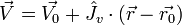
The wind vector field (u,v,w) as a function of altitude above some point (x₀,y₀) on the surface having an altitude z₀ is commonly referred to as the wind profile above that site. Conventionally, it is measured via radio sounding, whereas another approach to this is to use a remote sensing method. Depending on the wavelength of the radiation used, the scattering targets of interest are aerosols (in case of an IR heterodyne Doppler Lidar), air molecules (for an UV Doppler Lidar for observations in clear air, i.e. aerosol free), precipitation (for weather radar), or Bragg Scattering on refractive index variations due to turbulence eddies(for a radar wind profiler). If the respective tracer is moving with the velocity of the surrounding air, the backscattered signal will be shifted in frequency due to the Doppler effect. If this frequency shift is measured, the component of the velocity in the direction of the beam, the radial velocity V_r, is obtained. Using such a methodology, one gets the whole wind profile instantaneously, i.e. not one point at a time like in a radiosonde descent, and with a high update rate.

Considering the relationship of the radial component of the wind V_r in the direction of observation

$V_r=u \cdot\sin\theta\cos\phi+v\cdot\cos\theta\cos\phi+w\cdot\sin\phi$     Eq. 1

with the radar or lidar beam having an elevation angle $\phi$ and an azimuth angle $\theta$ (see figure 1) , three different directions of observation that are not coplanar are the minimum necessary to determine all three wind components.

Figure 1: Sketch of volume scan strategy showing the polar coordinate system being the basis for Eq. 1

4.3.2 Retrieval Algorithms and Errors

A scan strategy widely used by radar wind profilers and vertically pointing Doppler lidars is the Doppler Beam Swinging Technique (DBS), using for example four orthogonal azimuth directions at some elevation close to the vertical and a fifth measurement for the vertical itself. Another technique in this vein has been proposed by Lhermitte and Atlas for precipitation Doppler radars, but of course also applicable to every other dopplerized remote sensing technique, makes use of a full circle scan in azimuth (R.M. Lhermitte, D.A. Atlas, 1961; R.M. Lhermitte 1962). The technique is called Velocity Azimuth Display (VAD), since in the days when fast personal computers were not ubiquitous the horizontal wind and the particle fall velocity were extracted from the actual display of the range gated Doppler shift over azimuth (as an example see figure 2).

Figure 2: Example of a Velocity Azimuth Display, the corresponding radial wind field is shown in the small box

Although the trained observer may be able to extract also characteristics of inhomogeneous wind fields, the general approach would be to fit the parameters u, v and w (w being dominated by the fall velocity of rain drops in the case of weather radar) to Eq.1.

A refined version of the VAD analysis has been proposed by Browning and Wexler (K.A. Browning and R. Wexler, 1968) using more terms of a general Fourier expansion of the VAD graph.

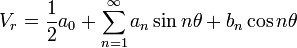$V_r=\frac{1}{2}a_0+\sum_{n=1}^\infty a_n\sin n\theta+b_n\cos n\theta$    Eq. 2

Assuming homogeneous fall speed of rain drops over the area of the VAD circle (or equivalently constant vertical velocity w), the following parameters can be expressed by the first Fourier coefficients (R: radius of the VAD circle). Note that Browning and Wexler used the normal mathematical definition of angles, not the meteorological, and therefore Eq. 5 differs slightly from their publication in that a₁ and b₁ are interchanged.

Horizontal divergence: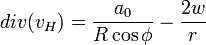$div(v_H)=\frac{a_0}{R\cos\phi}-\frac{2w}{r}$    Eq. 3

Horizontal wind speed: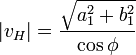$|v_H|=\frac{\sqrt{a_1^2+b_1^2}}{\cos\phi}$    Eq. 4

Wind Direction: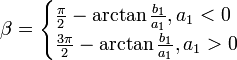$\beta=\begin{cases}\frac{\pi}{2}-\arctan\frac{b_1}{a_1},a_1<0 \\ \frac{3\pi}{2}-\arctan\frac{b_1}{a_1},a_1>0\end{cases}$    Eq. 5

Resultant deformation:$def_r(v_H)=-2\frac{\sqrt{a_2^2+b_2^2}}{R\cos\phi}$    Eq. 6

Combining the concept of a linear wind field ($\vec{V}$ : 3D wind vector, $\hat{J_v}$ : Jacobian matrix)

$\vec{V}=\vec{V_0}+\hat{J_v}\cdot(\vec{r}-\vec{r_0})$    Eq. 7

with a full volume scan, Waldteufel and Corbin suggested in 1979 the Volume Velocity Processing (VVP) Method (P. Waldteufel, H. Corbin, 1979) . When Eq. 8 is transformed to polar coordinates (r: Range) and inserted into Eq. 1 setting x₀ = y₀ = 0 it follows:

$\begin{align}V_r=u_0\cdot\sin\theta\cos\phi+v_0\cdot\cos\theta\cos\phi+w_0\cdot\sin\phi\end{align}$    Eq. 8

$\begin{align}+r\sin^2\theta\cos^2\phi\cdot u'_x \\ +r\cos^2\theta\cos^2\phi\cdot v'_y \\ +r\cos\theta\sin\theta\cos^2\phi\cdot (u'_y+v'_x) \\ +\sin\phi(r\sin\phi-z_0)\cdot w'_z \\ +\sin\theta\cos\phi(r\sin\phi-z_0)\cdot (u'_z+w'_x) \\ +\cos\theta\cos\phi(r\sin\phi-z_0)\cdot (v'_z+w'_y)\end{align}$

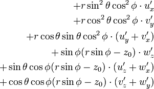
Thus, there are a maximum of nine parameters that can be obtained by fitting Eq. 8 to the volume velocity data for each altitude gate. As an example for one of these parameters, a plot of a vertical profile of the horizontal wind is shown in figure 3. Particularly for the horizontal wind, it is also common to plot wind barbs for each altitude gate. This can be conviently displayed as a time series (figure 4).

Figure 3: Profile of horizontal wind, similar plots could be shown for other paramters extracted from a volume scan by fittinbg Eq. 8 to it.

Figure 4: Time series of wind barbs as a function of altitude (time: abscissa, altitude: ordinate). This plot has the advantage that the direction of the horizontal wind can be displayed as well.

It is worthwhile noting that horizontal vorticity η (the vertical component of the curl of the velocity field, Eq. 9) cannot be extracted, since u'_y and v'_x only appear summed together.

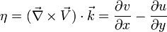$\eta=(\vec{\nabla}\times\vec{V})\cdot \vec{k} = {\partial v\over\partial x}-{\partial u\over\partial y}$, $\vec{k}$: unit vector in z-direction.    Eq. 9

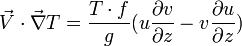
Since the assumption of a linear variation of the wind field is most likely to hold if the weather situation is stratified, it seems also sensible to set w'_x and w'_y to zero. Thus, profiles of the following meaningful properties can be obtained by the VVP method in addition to the wind profile: Divergence, vertical shear and Deformation. With regard to sensor synergies, temperature advection as a derived property might be of interest as well. Assuming pure geostrophic wind vg, i.e. the flow of air is devoid of any friction with the surface, gives rise for the following expression (see e.g. Holton 1992)

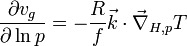${\partial v_g\over\partial \ln p}=-\frac{R}{f}\vec{k}\cdot\vec{\nabla}_{H,p}T$    Eq. 10

where T is the thermodynamic temperature, R the gas constant, f the Coriolis factor, and $\vec{\nabla}_{H,p}$ the horizontal Nabla Operator on isobaric surfaces. Using the ideal gas law, the following relation for the temperature advection holds (Rainbow® 5 instruction manual):

$\vec{V}\cdot\vec{\nabla}T=\frac{T\cdot f}{g}(u{\partial v\over\partial z}-v{\partial u\over\partial z})$    Eq. 11

However, if derivatives of the wind field are to be extracted in addition to the horizontal wind using VVP, one has to be aware that the corresponding matrix used in the fit is generally prone to be ill-conditioned, i.e. the solution varies too strongly with a variation of the arguments with respect to round-off errors due to the finite precision of floating point numbers, or, stated more formally, the condition number C given by the ratio of the largest and the smallest singular value of the matrix X^TX encountered in the least square fit procedure is too large, meaning roughly that log₁₀(C) is greater than the machine size precision (for more information see e.g. Wolfram Mathworld). For this reason, Nan et al. have suggested an algorithm called SVVP (S for “stepped”) to overcome this problem (Nan et al., 2007).

4.3.3 Performance

The methods presented here are not only different analysis methods, but also imply different scan strategies. Therefore, a trade-off has to be made in order to reconcile update rate, accuracy, representativeness and the possibility to obtain additional information about the nature of the wind field. For weather radars, wind profile quality has been compared by Holleman (Holleman, 2005) for different versions of VAD and the VVP methods. He used two different VAD methods (VAD1: Fourier expansion terminated after the third term, VAD2: Fourier expansion terminated after fifth term) and three different VVP methods with three, six and all nine parameters (VVP1: only wind profile (u₀,v₀,w₀); VVP2: divergence, stretching deformation and shearing deformation in addition to wind profile; VVP3: all parameters from VVP2 along with the vertical derivatives). In fact, only wind profiles obtained from VAD1 have been used for comparison with VVP1 and VVP2, since the single parameters have no effect on each other in value and magnitude of error due to the orthogonality of the basis functions of the expansion and the evenly spaced azimuthal intervals. This is of course not the case for the VVP methods. It must be noted, that the VAD data are not obtained from one azimuth circle, but from the same volume data as the VVP products. The difference is only that in the case of VAD the least square fit has been applied to all azimuth circles individually, whereas for the VVP product the volume data have been subjected to the fit at once. Therefore, the effect of using more data for the VVP than for the VAD is eliminated. During the study data from the KNMI C-band Doppler Weather Radar in DeBilt (Meteor AC360), Radiosonde launches in DeBilt and data from the HIRLAM model (Unden et al. 2002) have been compared for nine months. Products have been generated using the Rainbow® 5 software. The conclusion is that the VVP method is superior to VAD in general. Furthermore, the VVP1 method provides the best horizontal wind values which is attributed to noise fitting due to the non-orthogonality of the basis functions of the fit for VVP2 and VVP3 (and therefore linear dependencies between them). The VVP1 minus background statistics have been found to be at least as good as those of the radiosonde profiles.

4.4 Aerosol Backscatter and Extinction profile

Contributors: I. Mattis, D. Nicolae, O. Cox

The atmosphere contains a wide range of constituents extending from atoms and molecules (Angstrom range d ~ 1E-3 ... 1E-4 μm) to aerosols (d ~ 1E-2 ... 5 μm), cloud water droplets and ice crystals (d ~ 1 ... 15 μm and even larger). Evaporation, condensation, coagulation, absorption, desorption, and chemical reactions change the atmospheric aerosol composition on short timescales. Aerosol concentrations in the atmosphere vary widely with altitude, time, and location. The term “extinction” means the loss of light in the atmosphere from a directly transmitted beam. Two different mechanisms contribute to extinction: absorption and scattering. Aerosol extinction coefficient is a measure of attenuation of the light passing through the atmosphere due to the scattering and absorption by aerosol particles. Extinction coefficient is the fractional depletion of radiance per unit path length (also called attenuation especially in reference to radar frequencies). It has units of (1/km). The integrated extinction coefficient over a vertical column of unit cross section is called aerosol optical depth or optical thickness. Most of the aerosol particles are so weakly absorbing that their extinction is almost entirely due to scattering, rather than absorption. However, soot (carbon) particles are quite strong absorbers. Conform to the diffraction theory, an obstacle could be “seen” by an electromagnetic wave having a wavelength on the same magnitude as the geometric dimension of the obstacle. So, using a light beam (wavelength: nm, μm) one can detect atmospheric components, which are “invisible” for other sounding waves. The mixture of different components in the atmosphere results in a series of complex atmospheric interactions that take place with a laser beam:

• N2, O2 molecular elastic (λD = λL) light scattering; i.e. Rayleigh diffusion (λL >> d, where d is the molecular diameter)

• Aerosol elastic (λD = λL) light scattering; i.e. Mie scattering (λL ~ d, where d is the diameter of the particle)

• N2, O2 and H2O molecular inelastic (λD ≠ λR) light scattering; i.e. Raman scattering (λL >> d, with d the molecular dimension)

• Gas and aerosol absorption (if the radiation at λL is absorbed by atmospheric molecules or by compounds forming the aerosols

• Fluorescence of bioaerosols

Lidar makes use of a laser to excite backscattering in the atmosphere. This backscattered signal is observed using a telescope receiver, which collects the light and send it to the receiver optics. The role of the optical chain is to select specific wavelengths, split between them and direct them to photodetectors, which further convert the optical signal into electrical signals. These are recorded as a function of time by analog-to-digital converters and/or photon counting devices.

File:1.jpg

400px

Whatever the set-up of the lidar system, the magnitude of the received lidar signal is proportional to the number density of the atmospheric diffusers (molecules or aerosols), their intrinsic properties (i.e. probability of interaction with the electromagnetic radiation at the laser wavelengths, called cross–section value) and with the laser incident energy (Measures, 1992). Therefore, obtaining information about the aerosols means to find solutions of the equation which relates the characteristics of the received and emitted signal, and the propagation medium. The form of the equation depends of the interaction type. The basic lidar equation takes into account all forms of scattering and can be used to calculate the signal strength for all types of lidar, except those that employ coherent detection.

The detected light backscatter power S(λD,R) at the wavelength λD from a distance R can be expressed as follows (Nicolae, 2010):

where RCS is the range corrected signal 180px and CS is the instrument function . The atmospheric backscatter coefficient is a key element of the lidar equation, and is proportional to the cross section of the involved physical process and to the number density of the atmospheric active diffusers (i.e. atoms, molecules, particles, clouds) in the probed volume.

200px

220px and 220px are the atmospheric transmittance from the transmitter to the probed volume and from the probed volume to the receiver, respectively, where α(λ,R) is the atmospheric extinction coefficient and may be different on the two directions of the laser pulses, as is the case of the Raman backscatter radiation (λD = λR ≠ λL). The parameters α(λ,R), β(λ,R) and σ(λL,λD,R) refers to all possible physical interactions within the atmosphere. The backscattered radiation is usually detected at the laser wavelength (elastic processes) but the radiation shifted in wavelength, due to inelastic processes as the Raman effect, may be also detected. When the lidar equation is adapted to the specific process involved (i.e. Rayleigh, Mie, Raman), various atmospheric properties and parameters can be retrieved. Both in case of elastic backscatter lidar, and Raman lidar, the solution of the equation is not unique (Kovalev,2004), since it has two unknowns: backscatter and extinction coefficients. Combination of elastic and (vibrational) Raman channels allow to retrieve these parameters with minimum assumptions:

where the “L” and “R” indexes correspond to laser and Raman detected wavelength, respectively, and k ranges between 0.8 and 1.2. This relation is valid if the difference between the Raman and laser wavelength is small. Nitrogen molecules are used to obtain the Raman signal, due to the fact that Nitrogen is considered a gas with constant concentration over time and has a Raman spectra easy to be separated from the Rayleigh one. In this case, the second (532 nm) and third harmonics (355 nm) of Nd:YAG laser can be used as excitation, since the associated Raman lines are close to these wavelengths: 607 nm and 387 nm, respectively. With this hypothesis, the aerosol extinction coefficient at the laser wavelength can be obtained by applying the natural logarithm and the derivative to the Raman lidar equation:

320px

Molecular parameters (indices "m") can be calculated with sufficient accuracy from ground values of pressure and temperature using an atmospheric model, or radiosounding. A simple mathematical procedure applied to the couple elastic + Raman channel leads further to the retrieval of the backscatter coefficient (Mattis, 2002). With different couples of elastic and Raman channels, extinction and backscatter coefficients at several wavelengths can be computed, and therefore more products can be obtained (Müller,1999a): lidar ratios, Angstrom exponents, color ratios and even microphysical parameters such as size distribution, effective radius, complex refractive index, single scattering albedo, volume and number concentration.

4.5 Target classification

Contributors: E. O’Connor, M. Haeffelin, U. Görsdorf, JC. Dupont

4.5.1 Ceilometers

Contributors: M. Haeffelin

4.6 Mixing height

Contributors: M. Haeffelin, F. Angelini, R. Lehtninen, M. Piringer

4.6.1 Doppler lidars

Contributors: E. O'Connor

4.7 Liquid clouds

Contributors: G. Martucci, H. Russchenberg

4.7.1 Fundamentals

Both aerosols and clouds cause a direct radiative forcing by scattering and absorbing solar and infrared radiation in the atmosphere. The aerosol mass load along the atmospheric column as well as the aerosol optical thickness are integrated variables that can be used to infer the aerosol direct radiative effect. In the last century, with the global increase of their average load, aerosols have most likely made a significant negative contribution to the overall radiative forcing. In fact, the IPCC fourth assessment report (IPCC, AR4, 2007) provides a -0.5 ± 0.4 W m-2 cooling effect due to the anthropogenic component of the total aerosol in the atmosphere. Through their role as nuclei of condensation, aerosols also alter warm, ice and mixed-phase cloud formation processes by increasing droplet number concentrations and ice particle concentrations. They decrease the precipitation efficiency of warm clouds and thereby cause an indirect radiative forcing associated with these changes in cloud properties. At the global scale clouds increase the reflection of incoming solar radiation from 15% to 30% with an overall forcing of about -44 W/m2. On the other hand, the reduced cloud thermal emission below clear-sky values enhances the cloud greenhouse effect by about 31 W/m² thus determining a net cooling effect of about 13 W/m² (Ramanathan et al., 1989). The determination of the global cloud radiative forcing intended as the difference between the radiation budget components for cloudy conditions and clear-sky conditions is a challenging task which remains affected by a large uncertainty. The increase in global surface temperature of 0.6°C that occurred in the last century corresponds to a change of less than 1% in the radiative energy balance between short wave (SW) absorption and long wave (LW) emission from the Earth system (Kaufman et al., 2002). Despite the critical role of this energy mechanism, the balance between cooling and warming effect due to LW and SW net fluxes in cloudy regions remains one of the largest uncertainties when assessing the aerosol indirect effect, IE (Twomey, 1977). The reported observation that the greenhouse effect due to cloud is larger than the equivalent effect from a hundredfold increase in CO2 mixing ratio (Ramanathan et al., 1989) as well as the fact that hydrometeors size and concentration affect the cloud albedo are amongst the primarily reasons why in the last 50 years studying cloud microphysics became paramount in order to understand climate changes. The level of water vapour supersaturation and the number of cloud condensation nuclei (CCN) is also indirectly related to the cloud albedo. In polluted air the number of CCN is supposed to increase rapidly leading to increased CDNC (Twomey, 1977), nevertheless the efficiency in activating CCN into CDNC depends on a number of factors including CCN size, chemical compositions and cloud dynamics (updraft and downdraft). There are instead no evidences of the impact of the entrainment-mixing on the activation process, although recent studies indicate homogeneous and inhomogeneous mixing as depleting mechanism for CDNC formation especially in warm cumuli (e.g. Morales et al., 2011).

File:IPCC AR4 RadForcing.jpg

Figure 1: : Global average radiative forcing in 2005 (5 to 95% uncertainty ranges) with respect to 1750 for CO2, CH4, N2O and other important agents and mechanisms, together with the typical geographical extent (spatial scale) of the forcing and the assessed level of scientific understanding (LOSU). Courtesy of IPPC (AR4, 2007)

Global numerical models can improve the knowledge of cloud microphysics at both global and regional scales notwithstanding the large computational costs and the significant uncertainty at the smaller scales. On the other hand, numerical simulations at the regional and micro-scale (cloud-resolved scale) can resolve with explicit integration schemes and reduced computational costs the microphysical processes of cloud formation and lifetime allowing the assessment of the aerosol IE, but lose in representativeness at larger scales. Clouds and aerosols observations from networks of in situ and ground-based remote sensing instrumentation are detailed and usually better descriptions of the optical and microphysical processes than the numerical models but have limited and heterogeneous geographical cover, usually more representative of specific areas like Europe and North America. In situ measurements are usually accurate and represent a reference for the ground-based remote sensing retrieved microphysics. The need of a reference becomes important especially when the microphysics is retrieved by integrated profiles and combined methodologies using multiple sensors based on different assumptions leading to significant errors. However, in situ measurements of cloud products require in-cloud flights or radiosoundings which have high costs and can only be organized occasionally or with poor temporal resolution.

On the contrary, ground-based remote sensing instrumentation can provide the cloud microphysics with cost-effective and continuous measurements. One solution is to adopt an established reference from either in-situ observations or numerical simulations and to calibrate different retrieval techniques against the accepted reference. This is normally a two-step procedure based on (i) the calibration of different microphysical retrieval methods against the selected reference and (ii) the following iterative convergence of the calibrated methods to a common microphysics with minimized uncertainty. The literature shows that the use of synergistic information from passive and active co-located remote sensors can provide sufficient input data to retrieve the cloud microphysics based on a number of assumptions (characteristic of each method). An efficient system of measurements must ensure the operational retrieval of the main cloud microphysical variables such as cloud droplets number concentration (CDNC), effective radius ($R_{eff}$ ), liquid water content (LWC), cloud albedo and cloud optical depth (COD). Several studies in the last two decades presented different methodologies capable to retrieve the microphysics of liquid clouds by combining data from ground-based remote sensing instrumentation (Fox and Illingworth, 1997; Boers et al., 2000; Liljegren et al., 2001; Dong and Mace, 2003; Boers et al., 2006; Illingworth et al., 2007; Turner et al., 2007; Brandau et al., 2010; Martucci and O'Dowd, 2011). All together, these retrieval techniques provides the full set of required microphysical variables (i.e. LWC, CDNC, $R_{eff}$ , albedo and COD), however most of them can only provide a sub-set of variables which often prevents the calculation of the aerosols IE unless including significant parameterizations and introducing additional uncertainty.

4.7.2 Cloud Droplet Number Concentration

Contributors: G. Martucci

The size distribution of droplets in a liquid cloud can be determined by in-situ or laboratory studies using elctronic techniques involving the spectrometry of the samples and sorting of droplets into size bins characterized by specific number concentrations. An example of spectrometry technique is the Forward Scattering Spectrometer Probe - FSSP - it is an optical particle counters (OPCs) that detects single particles and size them by measuring the intensity of light that the particle scatters when passing through a light beam. As all in-situ measurements also the FSSP modifies the droplet size distribution by simply interacting with the droplets and can locally modify ceryain microphysical parameters like the level of supersaturation. Although very accurate the cloud droplets size distribution and number concentration (CDNC) measurement techniques are affected by errors and uncertainties of different nature and significance. A common and well-accepted way to calculate the droplet size distribution n(r) not involving direct measurements of the droplet distribution relies on mathematical parameterizations of the size distribution. According to Levin (1954), the size distribution of droplets in liquid clouds can be represented faithfully by a log-normal distribution like the one shown here,

$n(r)\,=\,\frac{N}{\sqrt{2\pi}\log{\sigma_g}} \exp{\bigg\{-\frac{(\log{r}-\log{r_g})^2}{2\log^2{\sigma_g}}\bigg\}}$,

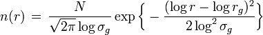where n(r) is the droplet number at radius r, N is the total number of droplets, $\sigma_g$ is the standard deviation of the log-normal distribution and $r_g$ its mean geometric radius. An alternative way to represent the droplet size distribution (DSD) is by a mono-modal gamma-type distribution. It is indeed convenient to adopt the already known and extensively used Gamma distribution (Boers and Mitchell, 1994) in the form of,

$n(r,z)\,=\,a(z)r(z)^{\alpha}\,\exp{(-b(z)r(z))}$

where n is the droplet concentration density, r is the radius of the droplets, b(z) is called rate parameter and a(z) is a function of the rate parameter and the Gamma function ($\Gamma(\alpha)$).

4.7.3 Effective Radius

Contributors: G. Martucci

The cloud droplets effective radius $R_{eff}$ is defined as the ratio of the third to the second moment of the DSD, n(r),

$R_{eff}\,=\,\frac{\int\limits_{0}^{\infty} n(r)\,r^3\operatorname{d}r}{\int\limits_{0}^{\infty} n(r)\,r^2\operatorname{d}r}$

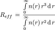
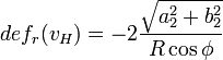
A practical way to express $R_{eff}$ takes into account the expression of n(r) in terms of the Gamma DSD by also combinig other calculations used in the past and current literature. Fox and Illingworth (1997) found an almost one-to-one relation between the RADAR reflectivity factor and reff. Based on this relation, reff can be expressed as the sixth root of the ratio between the detected RADAR reflectivity and the retrieved CDNC. Then, in case of Rayleigh approximation, the relation between $\langle r(z)^6\rangle$ and the RADAR reflectivity factor Z [mm6 m-3] is:

$\langle r(z)^6\rangle\,=\,\frac{Z(z)}{64\,N(z)}$,

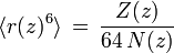Then, using the relation between the third and the sixth moment of the DSD and using the dependence on the DSD size parameter, $R_{eff}$ can be written as,

$R_{eff}\,=\,k_2^{-1}\,k_6^{-\frac{1}{6}}\,\bigg(\frac{Z(z)}{64\,N(z)}\bigg), \qquad k_2\,=\,\frac{\alpha^{\frac{1}{3}}\,(\alpha+1)^{\frac{1}{3}}}{(\alpha+2)^{\frac{2}{3}}}, \qquad k_6\,=\,\frac{(\alpha+3)\,(\alpha+4)\,(\alpha+5)}{\alpha\,(\alpha+1)\,(\alpha+2)}.$

The coefficients $k_2$ and $k_6$ depends on the shape parameter α and expresses the constant relation between the sixth and the third moment of the DSD.

4.7.4 Liquid Water Content

Contributors: G. Martucci

The degree of mixing that takes place between the uplifted cloudy air parcel and the drier environment controls the spatial (vertical) distribution of liquid water within a cloud. The cloud dynamics can then be extracted from a vertical profile of condensed liquid water through a cloudy layer especially if accompanied by a profile of temperature. Changes in the water content are paramount thermodinamically, as they lead to large energy changes. The precipitation is in fact strictly related to the temporal and spatial distribution of liquid water in the cloud. A thorough understanding of the mechanisms leading to the major themodynamic changes in the LWC facilitates an accurate calculation of the rate of growth of rain and drizzle drops as well as the assessment of ice crystal formation. This Section has for focus the liquid clouds especially the stratiform boundary layer clouds with negligible ice mass fraction. In these clouds the convection and the supersaturation values are well below the ones reached in the tropical and sub-tropical cumuli where the updraft and downdraft cycle dominates the thermodynacal effects on the LWC through the cloud.

File:INSITU LWC profile.jpg

Figure 2: : LWC by in-situ FAAM BAE-146, MACLOUD Inc, Mace Head, Ireland

For marine boundary-layer stratocumulus (Sc) clouds the LWC follows often a near-adiabatic or adiabatic profile between base and top of the cloud; aircraft in-situ measurements of marine Sc cloud above Mace Head (Ireland) during the MACLOUD field campaign (Decemeber 2010) show a typical LWC profile (Figure 2). In adiabatic conditions the LWC increases linearly from the base to the top of the cloud and can be expressed by the formula,

$LWC(z)\,=\,\frac{4}{3}\,\pi\,\rho_w\,N(z)\,\langle r(z)^3\rangle$.

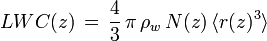The LWC is then proportional to the concentration of cloud droplets N (N indicates CDNC) and to the third moment of the DSD. Although the departure from purely adiabatic conditions is normally not significant for marine Sc, there are cases in which the adiabatic assumption leads to a significant overestimation of the total amount of water in the cloud and to inaccurate micriphysics. A linear modification of the above expression of the LWC includes the subadiabatic term $f(z)$. In fact, in order to provide a realistic representation of the liquid water profile through liquid clouds, the subadiabatic function $f(z)$ is considered to describe the adiabatic departure at each height z:

$LWC(z)\,=\,f(z)\,A_{ad}\,z$.

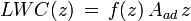This above expression for the LWC introduces the subadiabatic function $f(z)$ which depends on the height z along the cloud layer and that modifies the vertical gradient of the adiabatic LWC, $A_{ad}$, by providing the subadiabatic departure along the LWC profile.Different approaches to calculate the departure correction function f(z) have been suggested in the recent literature (Boers et al., 2000; Boers et al., 2006; Brandau et al., 2010, Martucci and O'Dowd 2011) and they all use the integrated for of the LWC retrieved by a microwave-radiometer to constraint the above equation and assess the calue of $f(z)$.

4.7.5 Liquid Water Path

Contributors: J. Gueldner

Figure 1: Histogram of MWP-derived LWP at Lindenberg observatory during 2010

The Liquid water path (LWP) can be measured by Microwave radiometer (MWR), Cloud radar and in the case of thin clouds by Infrared radiometer (Turner, 2007). The estimation of LWP by ground-based microwave radiometry has a long tradition. Westwater (1978) proposed a dual-frequency radiometer with channels at the wing of the water vapor line at 22.235 GHz and in the window region at 31.65 GHz to derive the Integrated water vapor (IWV) and the LWP of the atmosphere. First tests start in 1980. Details of the physical background are described in the MWR Fundamentals and in various reviews as e.g. Askne and Westwater (1986).

In summary, due to the nearly linear relation between TB and IWV as well as vs LWP, the integrated values can be derived by linear equations as follows:

IWV = a₀ + a * TB

LWP = b₀ + b * TB

where a and b denote the coefficient vector and TB the brightness temperatures of the radiometer. Regression coefficients are calculated mainly on the basis of training data sets consisting of concurrent TB and IWV/LWP values. Both TB and LWP are results of radiative transfer and cloud model calculations basing on a representative dataset of radiosonde observations. The dimension of TB increases from two to higher numbers at the end of last century.

Figure 2: Model and MWR LWP (top) and solar radiation balance (bottom) observed at Lindenberg observatory in January 2010

First multichannel radiometers were developed to retrieve vertical structures of thermodynamic variables. Closely related was an accuracy improvement of LWP retrievals achieved by multiple regression techniques or neural networks. Löhnert and Crewell (2003) have shown by numerical experiments that the use of additional channels at about 50 GHz and 90 GHz result in better retrievals. Compared to the classical two-channel algorithm the rms-error could be reduced from about 35 gm^-2 to 15-20 gm^-2. Therefore systematic errors due to different cloud model statistics became more important. Nevertheless, in spite of the technological progress uncertainties in LWP estimations remain unsettled. In a study (Turner et al., 2007) an identical data set of brightness temperatures was used to retrieve LWP by various methods and absorption models. The results are sensitive to the absorption models used as well as to the retrieval methods and cause biases of up to 40%. Hence, the combination of different active and passive sounding instruments is needed to meet user requirements. However, due to their capability to provide continuous observations, microwave derived LWP are widely used and well suited for a multitude of tasks:

• Long-term observations (Validation of new methods, climate applications)
  • Figure_lwp1 gives an impression about the amount of liquid water at Lindenberg during one year. It shows a histogram of non-rejected retrievals indicating that no liquid water was observed at about 24% of the cases. For only for 8% the LWP was greater than 200 gm^-2.

• Sensor synergy ( IPT, Cloudnet)

• NWP model validation:
  • For validation studies LWP measurements are needed as component of a variety of continuously observed parameters. Investigations, which aim at the revealing of possible deficiencies in the model parameterization, have to rely on the long-term availability of corresponding parameters. The periods may cover time intervals ranging from months up to several years. LWP from MWP can be provided for such long periods of time. In the frame of a validation study (Vogel et al., 2011, personal communication) of operational weather forecast models (IFS, COSMO-EU) a systematic prediction error of the 2 m temperature during winter months was found. The overestimation of the noon temperature results from an error of the radiation balance at surface of about 20-40 W m^-2. In order to find reasons for the overestimation the radiation balance was split into solar and thermal components. In fact, model radiation peaks appear in low stratiform clouds because their cloud water content is considerably to low compared to the MWP-derived LWP. Furthermore, if the model produces a realistic LWP then the radiance balance simulated by the IFS agrees with the observation (Figure).

4.7.6 Indirect effect

Contributors: G. Martucci, H. Russchenberg

The generally accepted way to quantify the radiative forcing due to clouds (cloud albedo forcing) is to study the change of representative cloud microphysical variables (e.g., $R_{eff}$) against a representative sub-cloud aerosol quantity (e.g., extinction). The cloud albedo depends on the cloud (geometrical and optical) thickness, the LWC and the CDNC and it is a way to express the amount of reflected and absorbed solar radiation by a cloud. The cloud albedo contributes then, as other indirect effects, to a global cooling by net removal of incoming solar radiation from the lower atmosphere (Seinfeld and Pandis, 1998; Ackerman et al., 2000, Zhao et al., 2012). McComiskey and Feingold (2007) have indicated that the radiative forcing of the aerosol indirect effects (IE), which is the difference in radiative flux that occurs as a result of changes in cloud properties for post- versus pre-industrial aerosol concentrations, ranges from -3 to -10 W m-2 for each 0.05 increment in IE ($\textstyle{IE\,=\,-\partial\ln{(R_{eff})}/\partial\ln{(\alpha})}$ , where $\alpha$ is the aerosol amount). Therefore, the accurate quantification of the aerosols IE is paramount for better prediction of climate change. In-situ airborne retrievals of the $R_{eff}$ and CDNC conducted in the past have facilitated the aerosols IE assessment with satisfactory accuracy (e.g. Brenguier et al., 2000). However, aircraft campaigns are costly, labour-intensive and not suited to long-term monitoring purposes. As described by Feingold and colleagues in 2001 and 2003, the combined retrievals of the sub-cloud aerosols optical properties (e.g., extinction, $\sigma$) and the cloud microphysics allow the assessment of the IE. Quantification of the IE using state-of-the-art techniques mainly relies on the inherent relation between the mean cloud droplet $R_{eff}$ and the sub-cloud value of $\sigma$,

$IE\,=\,-\partial\ln{(R_{eff})}/\partial\ln{(\sigma})$

The methodology behind eq.1 reflects the choice of using $\sigma$ as widely accepted proxy for the aerosols IE assessment to represent the generic aerosol amount $\alpha$; while this relation permits to quantify the aerosols IE not only by in-situ measurements but also using ground-based remote sensors, it exposes the aerosols IE quantification to the large uncertainty usually related to the $R_{eff}$ and $\sigma$ retrievals. Nevertheless, the successful calibration of the microphysics retrieval methods against an established and reliable reference leading to the convergence onto a common and more accurate microphysics by iterative evaluations would reduce the uncertainty associated to the microphysical variables and provide the bedrock for an even more advanced assessment of the IE. In fact, the general definition of the aerosols IE can be expressed by:

$IE\,=\,-\partial\ln{(C_{var})}/\partial\ln{(A_{var}})$,

Where $C_{var}$ and $A_{var}$ are the representative variables for cloud and aerosol amounts, respectively. A sensitivity analysis of the aerosols IE to new proxies can then be performed in order to further reduce the uncertainty affecting its quantification.

New proxies can be defined through:

$IE\,=\,-\partial\ln{(R_{eff})}/\partial\ln{(\sigma})$,

$IE\,=\,-\partial\ln{(N_{cloud})}/\partial\ln{(N_{cloud}})$,

$IE\,=\,-\partial\ln{(Z_{cloud})}/\partial\ln{(\sigma})$,

$IE\,=\,-\partial\ln{(R_{eff}^{\,cloud})}/\partial\ln{(R_{eff}^{\,aerosols}})$.

The IE values obtained from the above equations are affected by different types of uncertainty resulting from the errors related to the individual microphysical variables of both clouds and aerosols. This approach, also supported by the ACTRIS WP22 A framework for cloud-aerosol interaction studies, "aims to provide new recommendations to the scientific community about the development of new experimental means to quantify the indirect effects of aerosols. The need for unambiguous measurements of aerosols IE challenges the state-of-the-art remote sensing technologies of today and calls for the improvement of new observation methods". EG-CLIMET has provided the optimal scientific environment since February 2008 promoting proactive collaborations amongst the main European research groups in aerosols and cloud microphysics and facilitating the cuncurrent collaboration with other key European projects (e.g., ACTRIS, Paris-Fog, MWRNet) to achieve its objectives. EG-CLIMET created the coditions for a significant advance in the optimisation of cloud microphysical rertieval methods and, in pespective, in the quantification of the aerosols IE.

4.7.7 Available techniques

Contributors: G. Martucci, Ulrich Löhnert

The microphysical properties of boundary-layer liquid water clouds are essential for describing and predicting the development of the boundary layer, especially concerning their impact on radiative forcing, but also on atmospheric heating rates as well as the on the onset of precipitation (drizzle). Hence, it is imperative to assess currently used methods to derive the microphysics of liquid clouds in terms of CDNC, $R_{eff}$ and LWC and their related uncertainty. Within the scope of the COST action ES0702 EG-CLIMET four different ground-based remote sensing methods employing cloud radar, microwave radiometer (MWR) and laser-ceilometer have been developed and applied to model output and real measurement data. All methods use the same information on cloud phase & type, cloud boundaries, radar reflectivity, ceilometer-backscatter and MWR-derived LWP, respectively MWR brightness temperature.

File:Retrieval methods.jpg

Figure xxx: :EG-CLIMET state-of-the-art techniques to retrieve the microphysics from liquid clouds

Using this information as a common constraint, all four methods are applied to synthetic measurements calculated from model output using suited forward models available from the EarthCare Simulator. In this case retrieved microphysical properties can be directly compared to the original model output and thus the accuracy is evaluated as a function of height above cloud base. Systematic differences are assessed and it is shown that the CDNC and $R_{eff}$ retrievals are much more dependent on the retrieval method parameters than LWC. Additionally, the methods are applied to real measurements and evaluated through a short-wave radiative closure using simultaneous broad-band pyranometer measurements. For the initial calibration phase of the four different ground-based remote sensing methods intercomparison (Table 1) the retrieved cloud microphysics have been tested against the provided synthetic ECSIM (EarthCare Simulator)reference. Table 1 summarizes the state-of-the-art techniques retrieving the microphysics from liquid clouds. For each combination of instrument (Doppler cloud RADAR, LIDAR and microwave-radiometer) Table 1 shows: (2nd column) the name or acronym of the method and the main publication to which the method refers; (3rd column) the principles the methodology is based on; (4th column) the main assumptions and limitations/advantages of each method; (5th column) the availability to operate 24/7. The fourth column details the main advantages of the each method and its major sources of uncertainty, thus providing indications on where each technique can improve the accuracy of the retrievals. In brown colour are shown the methods involved in the "blind test" already in act within the scope of the COST action EG-CLIMET. The intercomparison, initially named blind test because the synthetic microphysical measurements remained unknown to the participants, led to a three-way intercomparison of the IPT-SYRSOC-TUD retrieval schemes with CLOUDNET not included in the initial intercomparison phase. For each microphysical variable (CDNC, $R_{eff}$, LWC) the outputs of the intercomparison yielded the (i) time-height timeseries of the difference between each method's retrieval and the ECSIM true value, and (ii) the mean variable profile over representative time intervals during the liquid cloud lifetime above the cloud base. The i-ii intercomparison outputs provide the uncertainty for each retrieval methods as compared to the true-measurements. The next session shows in details the results of the intercomparison outputs and related uncertainties.

4.7.8 Retrieval techniques and errors

Table 1 outlines the state-of-the-art retrieval techniques intercompared within the scope of the EG-CLIMET scientific program. The five retrieval methods are described hereafter.

4.7.8.1 SYRSOC- SYnergistic Remote Sensing Of Cloud

SYRSOC (SYnergistic Remote Sensing Of Cloud) is a multi-module technique developed at the National University of Ireland Galway and retrieving the three primary microphysical parameters from liquid clouds (Martucci and O’Dowd, 2011, Martucci et al., 2012, Ovadnevaite et al., 2011), i.e. the cloud droplet number concentration (CDNC), the effective radius ($R_{eff}$) and the cloud liquid water content (LWC). In addition to the three main microphysical variables, SYRSOC provides a number of parameters describing the cloud droplet spectral properties (relative dispersion), the degree cloud of subadiabaticity, the Doppler spectrum of droplets, the cloud optical depth and the cloud albedo. Extinction from standard 355-1500 nm inverted backscatter LIDAR signal or directly from Raman signal is used as input data for SYRSOC. Other input data are the temperature and humidity profiles from co-located operational microwave-radiometer and the reflectivity/signal-to-noise-ratio and depolarization ratio from co-located Ka-band Doppler cloud RADAR. Data from the 1064-nm and 15-km vertical range Jenoptik CHM15K LIDAR ceilometer, the RPG-HATPRO water vapour and oxygen multi-channel microwave profiler and the MIRA36, 35 GHz Ka-band Doppler cloud RADAR are currently used at the GAW Atmospheric Station of Mace Head (Ireland) to supply the necessary input to SYRSOC.

4.7.8.4 TUD-RSCPP - TU Delft Remotely-Sensed Cloud Property Profiles

The retrieval method relies on a combination of the cloud radar reflectivity; the microwave radiometer estimated liquid water path and on the cloud geometrical thickness from lidar and cloud radar. These observations are used as input data for different vertical cloud models to retrieve profiles of the LWC, the droplet concentration, the effective radius, the optical extinction and the optical depth. The three cloud models are characterized by their predefined in-cloud vertical structure of the assumed gamma DSD parameters (concentration, shape parameter and mean radius). This assumption is necessary to reduce the number of unknowns since the vertical information of the DSD properties from surface remote sensing observations are still lacking. The common assumptions in all three cloud models on the vertical distribution of the DSD parameters are that the cloud droplet concentration and DSD shape parameter remain constant within the cloud layer. The differences in the in-cloud vertical structure of the cloud models are related to the cloud layer mean droplet radius. In the vertical uniform (VU) cloud model, the cloud layer mean droplet radius is uniformly distributed over the cloud layer thickness while the scaled-adiabatic stratified (SAS) and homogeneous mixed (HM) cloud models parametrize the vertical profiles of the mean droplet radius in consideration of possible impacts of the cloud dilution. The SAS cloud model accounts for the entire range of mixing processes available in the atmosphere by a constant reduction in the particle size with height. In case of the HM cloud model, the impact of mixing is associated with the observed vertical variation in the radar reflectivity profile, which is attributed to changes in the mean particle size. The main assumptions constrain the application of the algorithms to liquid water clouds without drizzle formation and it is expected that drizzle-sized particles will produce biased results, because they are dominating the cloud radar reflectivity while their contribution to the LWC, the droplet concentration and the effective particle size are rather small.

4.7.8.5 G. Pace

• ECSIM vs Retr. Methods, ASTEX case, Effective Radius
• ASTEX SYRSOC-CLEAN-IV Reff prof 0-5.jpg
• BRANDAU ASTEX V3 2 Reff prof 0-5.jpg
• IPT ASTEX III Reff prof 0-5.jpg

4.8 Ice clouds

Contributors: D. Donovan, J. Delanoe, R. Hogan

5 Networks

Contributors: C. Gaffard, M. Haeffelin

5.1 Operational networks

Contributors:

5.1.1 CWINDE

Contributors:

CWINDE network managed by EUMETNET

5.1.2 CN-MET

Contributors: Dominique Ruffieux, Alexander Haefele

Main purpose of the CN-MET project (Centrale Nucléaire et METéorologie) is to bring up to date the system delivering weather information necessary to the population safety in case of a nuclear hazard. CN-MET represents the coupling of a specifically adapted measurement network and a predictive tool in the form of a fine grid numerical weather prediction model currently developed at MeteoSwiss (COSMO-2). This new tool, calling upon modern measurement and modeling techniques of the atmosphere, represents a solution which will keep all its relevance for the next decades.

In case of a nuclear accident, the necessary atmospheric data used to calculate the diffusion of a contaminated air mass will be provided by a fine grid numerical model, covering the whole Swiss territory. The new measurement network within CN-MET is directly adapted to provide the best information (initial and boundary conditions, and test measurements) for this model. CN-MET not only ensures the emergency preparedness for the concerned population on a local scale, but also enhances it on a regional scale corresponding to the Swiss Plateau.

More information at: Calpini, B., Ruffieux, D., Bettems, J.-M., Hug, C., Huguenin, P., Isaak, H.-P., Kaufmann, P., Maier, O., and Steiner, P.: Ground-based remote sensing profiling and numerical weather prediction model to manage nuclear power plants meteorological surveillance in Switzerland, Atmos. Meas. Tech., 4, 1617-1625, doi:10.5194/amt-4-1617-2011, 2011.

5.2 Candidate networks

Contributors:

5.2.1 Ceilometer network

Contributors:Martial Haeffelin, Owen cox

5.2.2 MWRNET

Contributors: N. Cimini, U. Löhnert

The International network of MicroWave Radiometers (MWRnet) aims to address the lack of coordination between the MWR operations in the world. The long-term mission of MWRnet is the set up of an operational network sharing good practices (in terms of procedures, formats, quality control, protocols, software, etc...) and life cycle of MWR data.

More information at: MWRnet website

5.3 Testbeds

Contributors:

5.3.1 Helsinki testbed

Contributors: Jani Poutiainen (Jani is in parental leave until September, unless we manage to get more information this part might remain just a link to the Heslinky test bed )

The Helsinki testbed project goals broadly consist of mesoscale weather research, forecast and dispersion models development and verification, demonstration of integration of modern technologies with complete weather observation systems, end-user product development and demonstration and data distribution for public and research community. Helsinki testbed

5.3.2 FUND

Contributors: Catherine Gaffard

There is little knowledge about the requirements for observations of very high resolution numerical weather prediction models, e.g. in the UK Met Office for 1.5 km grid length. So in order to address this, the Met Office intended to set up a dense network of profilers around London, see Fig. 1. for its Future Upper Air Networks Design (FUND) Project. This test-bed wanted to examine the provision of vertical profiles of not only wind, but also temperature humidity and cloud, with network spacing less than 200km, by setting three integrated profiler stations all using a wind profiler, a ceilometer, a radiometer, plus for 2 of them a cloud radar. This test-bed would have used some of the NREC facilities like Chilbolton Cloud radar and the mobile wind profiler from UFAM. This test-bed has partially started in summer 2009 but run out of resource in 2010.

• Lesson learned
• Output

5.4 Observatories

Contributors:

6 Examples of applications

Contributors:

6.1 NWP data assimilation

Contributors:

• Wind profiler impact

7 References

Contributors: N. Cimini, G. Martucci

Askne, J. and E.R. Westwater, 1986: A review of ground-based remote sensing of temperature and moisture by passive microwave radiometers. IEEE Trans. Geosci. Remote Sens., GE-24, 340-352.

Boers, R., Russchenberg, H., Erkelens, J., and V. Venema, 2000. J. Appl. Meteor., 39, 169-181

Boers, R., J. R. Acarreta, and J. L. Gras, 2006. J. Geophys. Res., 111, D22208, doi: 10.1029/2005JD006838

Brandau, C.L., Russchenberg, H.W.J., Knap, W.H., 2010. Atmospheric Research, 96, DOI:10.1016/j.atmosres.2010.01.009.

Browning, K.A. and R. Wexler, 1968: The Determination of Kinematic Properties of a Wind Field Using Doppler Radar, J. Appl. Met., 7, 105-113.

Dong, X., and G.G. Mace, 2003. J. Atmos. and Oceanic Tech., 20, 42-53.

Fox, N. I., and A. J. Illingworth. J. Appl. Meteor., 36, 485-492, 1997

Kaufman, Y. J., D. Tanré, and O. Boucher, 2002. Nature, 419, 215–223.

Holleman I., 2005: Quality Control and Verification of Weather Radar Wind Profiles, J. Atm. Oc. Tech., 1541-1550.

Holton, J.R., 1992 (2005): An Introduction to Dynamic Meteorology, fourth edition, Elsevier Academic Press, ISBN: 0-12-354015-1.

Illingworth, A.J., R.J. Hogan, et al. 2007. Bull. Amer. Meteor. Soc., 88, 6, 883-898.

Kovalev V., V. Eichinger, Elastic Lidar. Theory, Practice, and Analysis Methods, Wiley Interscience Publ., New York, USA, 2004.

Lhermitte, R.M. and D. Atlas, 1961: Precipitation Motion by Pulse Doppler Radar in Measurements of Particle Fall Velocities, Proceedings of the 9th Weather Radar Conference, Boston, American Meteorological Society, 218-233.

Lhermitte, R.M., 1962: Note on Wind Variability with Doppler Radar, J. Atmos. Sci., 19, 343-346.

Liljegren, J.C., E. E. Clothiaux, G. G. Mace, S. Kato, and X. Dong, 2001. J. Geophys. Res., 106,

Löhnert, U. , S. Crewell, C. Simmer, 2004. Journal of Applied Meteorology, 43, No. 9, 1295-1307

Löhnert,U. and S.Crewell, 2003: Accuracy of cloud liquid water path from groud-based microwave radiometry. Part I. Dependency on cloud model statistics. Radio Sci. 38, 8041, doi:10.1029/202RS002654.

Measures R. M., Laser Remote Sensing. Fundamentals and Applications, Krieger Publishing Company, Malabar, Florida, 1992.

Martucci, G., J. Ovadnevaite, D. Ceburnis, H. Berresheim, S. Varghese, D. Martin, R. Flanagan, C.D. O’Dowd, 2012. Atmospheric Environment, 48C, 205-218.

Martucci, G. and O'Dowd, C. D., 2011. Atmos. Meas. Tech., 4, 2749-2765, doi:10.5194/amt-4-2749-2011.

Mattis I., et al., 2002: Geophys.Res. Let. 29, 1306.

Müller D., Wandinger U., Ansmann A., 1999: Appl Optics, 38, 2346.

Nan, L., W. Ming, T. Xiaowen, and P. Yujie, 2007: An Improved Velocity Volume Processing Method, Adv. Atmos. Sci., 24, 893-906.

Nicolae D., C. Talianu, T. Trickl, B. Tatarov, H. Nakane, N. Sugimoto, I. Serikov, V. Rizi, M. Iarlori, J. Pelon, P. Flamant, J. Spinhirne, Recent Advances in Atmospheric lidars, INOE Publishing House, 2010

Nicolae D., Belegante L., Nemuc A., 2010: Optoelectron. Adv. Mat.-RC, 4, 12.

Ovadnevaite, J., D. Ceburnis, G. Martucci, J. Bialek, C. Monahan, M. Rinaldi, M. C. Facchini, H. Berresheim, D. R. Worsnop, and C. O'Dowd, 2011. Geophys. Res. Lett., 38, L21806, doi:10.1029/2011GL048869

Solomon, S.; Qin, D.; Manning, M.; Chen, Z.; Marquis, M.; Averyt, K.B.; Tignor, M.; and Miller, H.L., ed., IPCC AR4 WG1: Climate Change 2007: The Physical Science Basis, Contribution of Working Group I to the Fourth Assessment Report of the Intergovernmental Panel on Climate Change, Cambridge University Press, ISBN 978-0-521-88009-1 (pb: 978-0-521-70596-7).

Rainbow® 5 Instruction Manual, Release 5.31.0: Products and Algorithms, Selex Systems Integration GmbH, Document Code: GEMA-SD-0150-5310-2.

Ramanathan, V., Cess, R. D., Harrison, E. F., Minnis, P., Barkstrom, B. R., Ahmad, E., and D. Hartmann, 1989. Science, 243 (4887), 57-63 [doi: 10.1126/science.243.4887.57]

Turner, D.D., 2007: Improved ground-based liquid water path retrievals using a combined infrared and microwave approach, J. Geophys. Res., 112, D15204, doi:10.1029/2007JD008530.

Turner, D.D., Vogelmann, A.M., Austin, R., Barnard, J.C., Cady-Pereira, K., Chiu, C., Clough, S.A., Flynn, C.J., Khaiyer, M.M., Liljegren, J.C., Johnson, K., Lin, B., Long, C.N., Marshak, A.,Matrosov, S.Y.,McFarlane, S.A., Miller,M.A., Min, Q., Minnis, P., O'Hirok, W., Wang, Z., Wiscombe, W. , 2007. Bull. Amer. Meteor. Soc., 88, 177–190.

Twomey, S.A.,1977. J. Atmos.Sci., 34, 1149-1152.

Unden, P., and Coauthors, 2002: Hirlam-5 scientific documentation, SMHI Hirlam-5 Project Tech. Rep., 146.

Waldteufel, P., and H. Corbin, 1979: On the analysis of single Doppler radar data, J. Appl. Meteor., 18, 532–542.

Westwater, E.R., 1978: The accuracy of water vapor and cloud liquid determination by dual-frequency ground-based microwave radiometry. Radio Sci 13, 667-685.

Wolfram Mathworld, http://mathworld.wolfram.com/ConditionNumber.html

Zhao C, SA Klein, S Xie, X Liu, JS Boyle, and Y Zhang. 2012. Geophysical Research Letters, 39, L08806, doi:10.1029/2012GL051213