Doppler beam swinging (DBS)
At least three linear independent beam directions and some assumptions concerning the wind field are required to transform the measured 'line-of-sight' radial velocities into the wind vector. Comparisons of RWP winds with data from a meteorological tower (Adachi et.al., 2005) and balloon soundings (Rao et.al. 2008) have shown that a four-beam based DBS sampling configuration is superior over a three-beam configuration in terms of data quality.
Cheong et.al. (2008) have found that the RMS error of RWP measurements can be significantly reduced by increasing the number of off-vertical beams in DBS beyond four. At present, such a configuration can only be used by a few RWP's systems because of restrictions imposed by the simple phased array constructions that are mostly used.

For a five-beam system and a (horizontally) constant wind field, the relation between wind vector and the 'line of sight' radial wind components is given by the following linear system:
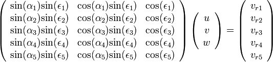
where  and
and  denote azimuth and elevation angles of beam
  . In compact matrix
notation, this can be written as
. In compact matrix
notation, this can be written as
 .
.
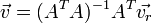
This over-determined system can be solved in a least-squares sense and the wind vector components can be obtained from the measured radial velocities through a pseudo-inverse as (the matrix superscripts T and 1 denote transposition and inverse, respectively).:
The homogeneity condition is of course not always fulfilled, in particular not in a convective boundary layer or in patchy precipitation. A discussion of the DBS method can be found in Koscielny et.al. (1984), Weber et.al. (1992), Goodrich et. al. (2002). The problem and the resulting measurement errors have recently been investigated by Scipion et.al. (2009), they are even noticeable in NWP data assimilation (Cardinali, 2009). However, the assumption is usually assumed to be correct for winds averaged over a longer time interval. Cheong et.al. (2008) have used data obtained with a volume-imaging multi-signal wind profiler in a convective boundary layer to show that for this particular case the assumptions inherent in the DBS method were valid for a wind field averaged over 10~minutes. This is the main reason why DBS RWP wind measurements are typically averages over 10-60~minutes. More work is required to obtain reliable quantitative estimates of this error under a variety of atmospheric conditions.